Discrete Probability Distributions with MS-Excel

Hi ML Enthusiasts! Today, we will talk about discrete probability distributions and their implementation in MS-Excel. This is very important as it lays the foundation of statistics which is very useful if you want your career in Data Science.

So, let’s get started!

Random Variables and their Types

Every experiment that we do has its associated outcomes. For example, tossing a coin has two outcomes, head and tail. Similarly, rolling a die has six outcomes, 1, 2, 3, 4, 5 and 6 dots. These outcomes are required to be defined using numerical values. This requirement is solved by using random variables.

Random variables serve the purpose of defining the experimental outcomes using numerical values. These numerical values can be discrete or continuous depending upon their properties. When the values the random variable takes have definable infinite range or gap or are finite in nature, such as 1, 2, 3, 4, …, n, it is called as discrete random variable. When the values do not have any definable range or gap, it is called as continuous random variable.

An example of discrete random variable is number of cars sold per day in a particular showroom. This random variable can take values such as 1, 2, 3, or more depending upon the number of cars sold per day. Also, there is a fixed gap between two numbers (2 – 1 = 4 – 3= 1). An example of continuous random variable is the values of temperature recorded after every one hour each day. For example, 22.6ºC, 26.44ºC etc.

Concept of Probability Distributions

Every value of random variable has a probability (likelihood of occurrence) associated with it. Probability distribution is defined as the description of how the probabilities are distributed over the different values the random variable takes.

Let the random variable be x. The probability function of x is defined as f(x). f(x) provides the curve of variation of probabilities with variation of x. For example, f(0) provides the probability of selling 0 cars per day, f(3) provides the probability of selling 3 cars per day. Likewise, f(0ºC) provides the probability that the temperature is 0ºC per hour.

Discrete Probability Distributions

When the random variable in consideration is discrete in nature, the probability distribution also comes out to be discrete. The required condition associated with it are as follows:

1 ≥ f(x) ≥ 0 and ∑f(x) = 1.

Following observations can be carried out from these two equations:

• The probability of the random variable can be greater than or equal to 0 and can be less than or equal to 1.
• The probability of a certain outcome is 1 and the probability of impossible outcome is 0. Thus, for certain outcome, f(x) = 1 and for impossible outcome, f(x) = 0.
• If the outcomes are random in nature, without any bias, having equal chance, then second equation holds true.

Implementation using MS-Excel

Now let’s learn how to analyse a discrete probability distribution on Excel.

Let’s consider a situation in which we are given the data of number of cars sold per month by a showroom and we need to come out with the probability distribution of this data.

• Please note that we can make our own data by using RAND() function of excel. It usually gives the output between 0 to 1.

• You can generate realistic numbers by first multiplying rand() by 100 and then using =int(100*rand()) in a cell and pressing enter key.

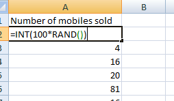
• The int() function does as expected, it converts the float output of the 100*rand() into nearest integer.
• In this way, you can generate any number of observations of your choice by dragging  “⌋” of the cell.

• I have generated 20 observation by dragging the cell up to 21st row as I have taken 1st row as the title row.
• You can get the total number of cars sold by using the sum() function of excel. Type =sum( in excel. Then, select the cell you want to take the data from (B2 in my case). Then press control+Down key. The selector will move towards the last cell of the column. Press control+shift+Up key to select all the rows/observations from the column and press enter. This produces the total number of cars sold in 20 months.
• Go to next column. Name the C1 cell as Probability of each outcome. You can get the probability value by dividing the particular number of cars sold column by total number of cars sold column as shown below:

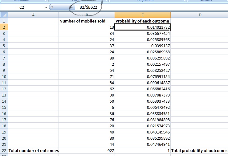
• Drag the cell formula down till your last cell to find out the probability of each of the outcomes. The sum of all the probabilities comes out to be equal to 1 and can be calculated using the previous approach.
• To make the probability distribution plot, select both the columns, Column B and C. Press on Insert button, go to Scatter and select Scatter with only markers.
• This will generate a scatter chart. Tap on that chart, go to Layout, add the title using Chart title, axis titles using Axis Titles and legend from Legend option. You will get a chart similar to this:

• So, this is the probability distribution plot of our situation. Note that, here, f(x) is between 0 and 1 and if we sum all the values of f(x), we get 1.

With this, we conclude our tutorial. We will talk about different types of discrete probability distributions in our next tutorial. So, stay tuned in this excel series.