

Perceptron
Perceptron is the first step towards learning Neural Network. It is a model inspired by brain, it follows the concept of neurons present in our brain. Several inputs are being sent to a neuron along with some weights, then for a corresponding value neuron fires depending upon the threshold being set in that neuron. For understanding the theory of Perceptron please go through our article on The Perceptron: A theoretical approach.
Algorithm of Perceptron
The perceptron algorithm is divided into three phases:
- Initialization phase : In this phase, we set the weights to any random values. They can be positive or negative.
- Training phase:
- For T iterations
- For each input vector
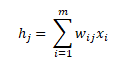
- Forward Propagation: Compute the activation and predicted outputs using the following equations:
- For each input vector
- For T iterations

Backward Propagation: Update the weights using the following equation:

- Recall Phase: Compute the activation of the neuron j using the final weights using the following equations:
Backpropagation
It is a method for calculating the errors when values of Activation function and Target values mismatch. By using Backpropagation we will automatically update weights. For example:
- Consider output of Activation function is A(i) and Target Value is T(i)
- Calculate error between A and T, that is, ‘A(i) – T(i)’
- Let Input vector corresndin to above A(i) is x(k).
- Weighted Error W_error(k,i) = (A(i) – T(i)) * x(k)
- New_weight = Old_weight + (eta) * W_error
‘eta’ is the Learning Rate. It helps in controlling the rate of change in Weights. Sometimes the system gets unstable if weights change very rapidly and it never sets down, in such scenarios we use Learning Rate (eta). Typically we take eta as (0.1 < eta < 0.4).
Now whenever we get any kind of mismatch in the Activation and Target values, we do Backpropagation to update our weights.
import numpy as np

values=([2.7810836,2.550537003],
[1.465489372,	2.362125076],
[3.396561688,	4.400293529],
[1.38807019,1.850220317],
[3.06407232,3.005305973],
[7.627531214,	2.759262235],
[5.332441248,	2.088626775],
[6.922596716,	1.77106367],
[8.675418651,	-0.242068655],
[7.673756466,	3.508563011])

print("Training input values without Bias\n", values)
Adding Bias to the Input Matrix
Bias value is like a cheat code to make training more reliable, now we will add biad value to Input matrix using ‘concatenate()’ method of numpy library.
test2 = [[-1]] * len(values)
values = np.concatenate((test2, values), axis = 1)
print("Training input values with bias in it\n",values)
Creating Random Weights
We will generate random values of weights for Weight vector, using ‘rand()’ method of numpy library. Size of Weight vector will be equal to total number of values in a row of Input vector. In our case it is ‘3’, including bias value.
m=3     #number of elements in each row of inputs
n=1
weights = np.random.rand(m,n)*0.1 - 0.5
print("Initial random weights\n",weights)
Target values Matrix
final = ([[0],[0],[0],[0],[0],[1],[1],[1],[1],[1]])
print("Training data target values are\n", final)
Method for updating Weights
If the value of Activation function is not equal to Target value, then we will use this method to update weights. We have introduced a new variable too, that is, Learning Rate (eta). It helps in controlling the rate of change in Weights. Sometimes the system gets unstable if weights change very rapidly and it never sets down, in such scenarios we use Learning Rate (eta). Typically we take eta as (0.1 < eta < 0.4). In our case we are taking it ‘0.25’
def updateWeights(weights, inputs, activation, targets):
    eta = 0.25
    weights += eta*np.dot(np.transpose(inputs), targets - activation)
    return weights
Creating method for Learning
This method calculates the Activation value and compares it with Target values, if they mismatch then the ‘updateWeights()’ method is being called to update weigts, then further Activation values are being calculated.
def  prediction (inputs, weights, targets):
    #representing Activation function with 'ack [[]]' variable
    ack = [[0]] * len(inputs)
    for i in range(0, len(inputs)):
        for j in range(0,len(weights)):
            ack[i] += inputs[i][j] * weights[j]
        ack[i] = np.where(ack[i]>0, 1, 0)
        #checking values with target
        if(targets[i] != ack[i]):
            weights = updateWeights(weights, inputs, ack[i], targets)
        print(ack[i])
    return weights
Training our model and extracting stable weights
Now we will do the training of our model, to do so we will use all the above data and methods and wil execute ‘prediction()’ method for ‘4’ times or until the Activation value gets equal to Target values and weights become stable.
iterations = 4
for temp in range(0, iterations):
    print("\nIteration ",temp+1,"\n")
    weights = prediction(values, weights, final)

print("\nTrained Weights\n", weights)
Testing our own data (Recall)
We will provide some data and our Perceptron will provide us some result corresponding to it. For this we will use Trained Weights that we extracted in above part and a new method ‘perceptronPredict()’
def perceptronPredict(weights, newInput):
    activation = np.dot(newInput, weights)
    activation = np.where(activation>0, 1, 0)
    print(activation)


newInput = ([-1.0, 1.786745, 2.94569],
            [-1.0, 7.023323, 1.9999])
perceptronPredict(weights, newInput)
Hence we got the results corresponding to each Input vector that we have supplied in the form of ‘newInput’ matrix.
Above post gave us an insight that how a basic Neural Network works and how it does the learning. In our next post we will learn a Multi-layer Neural Network!!
So stay tuned and keep learning!!!


Reblogged this on Qamar-ud-Din.