

PAM Clustering using R
Hi All!
Today, we will be learning how to perform PAM Clustering using R to achieve customer segmentation. This case-study comes under unsupervised machine learning (PAM or Partition Around Medoids Clustering).
Problem Statement
Being an owner of a mall, You want to understand how you can obtain different customer segments to know who can be your target customers so that you can inform your marketing team regarding your findings and can ask them to devise new strategies accordingly.
Data-set used
We will using Mall-Customers.csv file that can be found here on Kaggle. The data-set has the following variables:
- CustomerID: Unique ID assigned to the customer
- Gender: Gender of the customer
- Age: Age of the customer
- Annual Income: Annual Income of the customer
- Spending Score: Score assigned by the mall to the customer based on his/her spending history and sentiments.
Algorithm used
PAM Clustering
Language used
R
Algorithm Description
- Select k objects from the data-set to be set as k medoids.
- If, some k objects are already marked to be used as medoids, use them as medoids in the data-set.
- Calculate the dissimilarity matrix
- Assign other objects to their closest medoids.
- For each cluster, if you find any object that can reduce the average dissimilarity co-efficient, use it as that cluster’s medoid. Also, that object should be chosen as medoid which decreases the average dissimilarity co-efficient the most.
- If you find new medoid, go back to step 4 and reiterate till you don’t get any new medoid.
Distances used
In order to create the distance matrix in PAM, we can use the following two distances:
- Euclidean distance: This distance is the root of sum-of-squares of the differences.
- Manhattan distance: This distance is the sum of absolute differences.
When to use what distance?
- If the data you are having contains outliers, manhattan distance is much better in that case that Euclidean distance. This is because Euclidean distance is going to amplify that distance unusually due to the squares done to obtain it. Manhattan distance uses absolute distances so this is more robust to outliers.
- If outliers are not the cause of concern, then use any of them. They will be producing the same results.
Why PAM?
The method of finding mean in K-means algorithm is highly sensitive to outliers. This results in incorrect assignment of objects or observations to different clusters. The K-medoids or PAM clustering is highly robust to outliers.
The Code
Data Importing
We will start the analysis by importing the data.
rawdata = read.csv("Mall_Customers.csv")
head(rawdata)
## CustomerID Gender Age Annual.Income..k.. Spending.Score..1.100.
## 1 1 Male 19 15 39
## 2 2 Male 21 15 81
## 3 3 Female 20 16 6
## 4 4 Female 23 16 77
## 5 5 Female 31 17 40
## 6 6 Female 22 17 76Data Pre-processing
Let’s now fetch the summary of the data to see the descriptive statistics and the count of missing values.
colnames(rawdata) = c("CustomerID", "Gender", "Age", "Annual_Income", "Spending_Score")
data = rawdata
summary(data)
## CustomerID Gender Age Annual_Income
## Min. : 1.00 Length:200 Min. :18.00 Min. : 15.00
## 1st Qu.: 50.75 Class :character 1st Qu.:28.75 1st Qu.: 41.50
## Median :100.50 Mode :character Median :36.00 Median : 61.50
## Mean :100.50 Mean :38.85 Mean : 60.56
## 3rd Qu.:150.25 3rd Qu.:49.00 3rd Qu.: 78.00
## Max. :200.00 Max. :70.00 Max. :137.00
## Spending_Score
## Min. : 1.00
## 1st Qu.:34.75
## Median :50.00
## Mean :50.20
## 3rd Qu.:73.00
## Max. :99.00Let’s add dummy variables for gender now.
data$IsMale = ifelse(data$Gender=="Male", 1, 0)
data$IsFemale = ifelse(data$Gender=="Female", 1, 0)
data = data[, 3:ncol(data)]
head(data)
## Age Annual_Income Spending_Score IsMale IsFemale
## 1 19 15 39 1 0
## 2 21 15 81 1 0
## 3 20 16 6 0 1
## 4 23 16 77 0 1
## 5 31 17 40 0 1
## 6 22 17 76 0 1Let’s also examine the histograms of the data.
library(psych)
multi.hist(data,nrow = 3, ncol=2,density=TRUE,freq=FALSE,bcol="lightblue",
      dcol= c("red","blue"),dlty=c("solid", "dotted"),
main=colnames(data)) 

From above plot, we can see that Annual_Income and Age are left skewed. Spending score is nearly normal. IsMale and IsFemale are bimodal distributions.
PAM clustering using R
For cluster analysis and graphical representation of clusters, we will be using cluster and factoextra libraries of R.
library(cluster)
library(factoextra)
## Loading required package: ggplot2##
## Attaching package: 'ggplot2'## The following objects are masked from 'package:psych':
##
## %+%, alpha## Welcome! Want to learn more? See two factoextra-related books at https://goo.gl/ve3WBaNow, let’s examine the pam function to go ahead with this analysis. If you type ?pam in the R console, you’ll be able to get the documentation of pam, which parameters it take, what are the default arguments to those parameters etc. The main paramters of our interest are: pam(x, k,metric =“euclidean”,stand =FALSE)
x = numeric data or distance matrix obtained from daisy() or dist() k = number of clusters metric = which type of distancing you want to use – it can be either euclidean or manhattan stand = logical; if true, the measurements in x are standardized before calculating the dissimilarities. Measurements are standardized for each variable (column), by subtracting the variable’s mean value and dividing by the variable’s mean absolute deviation. If x is already a dissimilarity matrix, then this argument will be ignored
From above description, we can see that the value of k has to be provided as input to this function to obtain PAM clustering. The question which now arises is how to obtain the optimal number of clusters to be provided as input to k in pam function.
For this, we will have to do silhouette analysis.
scaleddata = scale(data)
fviz_nbclust(scaleddata, pam, method ="silhouette")+theme_minimal()
From above plot, we can see that the optimal number of clusters is k = 2. Let’s now start PAM clustering for k = 2.
pamResult <-pam(scaleddata, k = 2)
pamResult
## Medoids:
## ID Age Annual_Income Spending_Score IsMale IsFemale
## [1,] 78 0.08232511 -0.2497647 -0.08519365 1.1253282 -1.1253282
## [2,] 113 -0.06084899 0.1309742 -0.31753996 -0.8841865 0.8841865
## Clustering vector:
## [1] 1 1 2 2 2 2 2 2 1 2 1 2 2 2 1 1 2 1 1 2 1 1 2 1 2 1 2 1 2 2 1 2 1 1 2 2 2
## [38] 2 2 2 2 1 1 2 2 2 2 2 2 2 2 1 2 1 2 1 2 1 2 1 1 1 2 2 1 1 2 2 1 2 1 2 2 2
## [75] 1 1 2 1 2 2 1 1 1 2 2 1 2 2 2 2 2 1 1 2 2 1 2 2 1 1 2 2 1 1 1 2 2 1 1 1 1
## [112] 2 2 1 2 2 2 2 2 2 1 2 2 1 2 2 1 1 1 1 1 1 2 2 1 2 2 1 1 2 2 1 2 2 1 1 1 2
## [149] 2 1 1 1 2 2 2 2 1 2 1 2 2 2 1 2 1 2 1 2 2 1 1 1 1 1 2 2 1 1 1 1 2 2 1 2 2
## [186] 1 2 1 2 2 2 2 1 2 2 2 2 1 1 1
## Objective function:
## build swap
## 1.647591 1.647591
##
## Available components:
## [1] "medoids" "id.med" "clustering" "objective" "isolation"
## [6] "clusinfo" "silinfo" "diss" "call" "data"Let’s now bind the cluster data to the main dataframe.
rawdata$cluster = pamResult$cluster
head(rawdata)
## CustomerID Gender Age Annual_Income Spending_Score cluster
## 1 1 Male 19 15 39 1
## 2 2 Male 21 15 81 1
## 3 3 Female 20 16 6 2
## 4 4 Female 23 16 77 2
## 5 5 Female 31 17 40 2
## 6 6 Female 22 17 76 2pam function results and object of class pam which has two most important components: * medoids * clustering
Let’s examing them now.
pamResult$medoids## Age Annual_Income Spending_Score IsMale IsFemale
## [1,] 0.08232511 -0.2497647 -0.08519365 1.1253282 -1.1253282
## [2,] -0.06084899 0.1309742 -0.31753996 -0.8841865 0.8841865pamResult$clustering## [1] 1 1 2 2 2 2 2 2 1 2 1 2 2 2 1 1 2 1 1 2 1 1 2 1 2 1 2 1 2 2 1 2 1 1 2 2 2
## [38] 2 2 2 2 1 1 2 2 2 2 2 2 2 2 1 2 1 2 1 2 1 2 1 1 1 2 2 1 1 2 2 1 2 1 2 2 2
## [75] 1 1 2 1 2 2 1 1 1 2 2 1 2 2 2 2 2 1 1 2 2 1 2 2 1 1 2 2 1 1 1 2 2 1 1 1 1
## [112] 2 2 1 2 2 2 2 2 2 1 2 2 1 2 2 1 1 1 1 1 1 2 2 1 2 2 1 1 2 2 1 2 2 1 1 1 2
## [149] 2 1 1 1 2 2 2 2 1 2 1 2 2 2 1 2 1 2 1 2 2 1 1 1 1 1 2 2 1 1 1 1 2 2 1 2 2
## [186] 1 2 1 2 2 2 2 1 2 2 2 2 1 1 1Let’s now visualize our clusters.
fviz_cluster(pamResult,
             palette =c("#007892","#D9455F"),
             ellipse.type ="euclid",
             repel =TRUE,
             ggtheme =theme_minimal())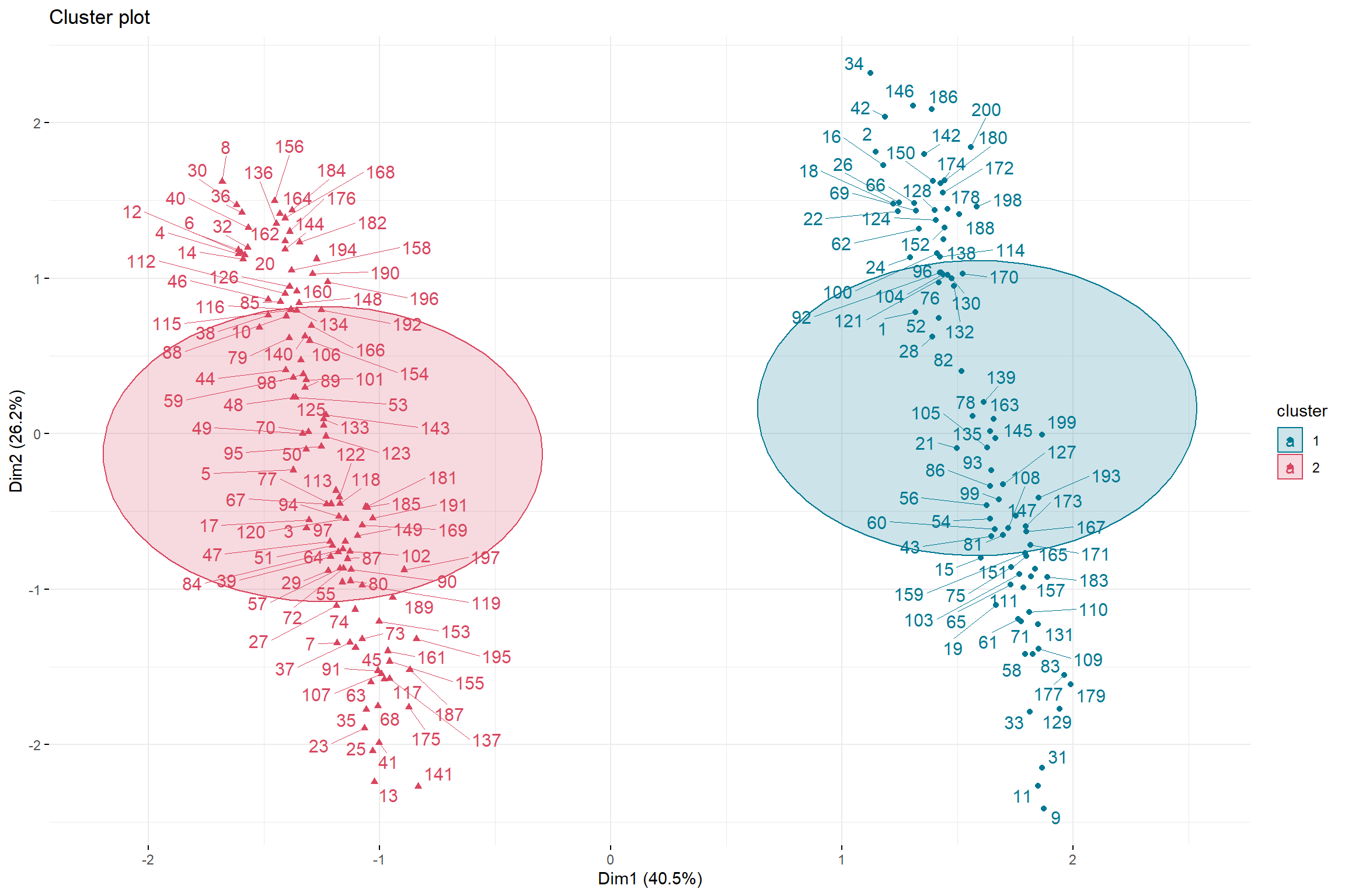
So guys, with this, I conclude this tutorial on PAM clustering with R.
Stay tuned for more such interesting case-studies. Also, don’t forget to check out our YouTube channel, ML for Analytics.


