
Hi ML enthusiasts! In our last post, we talked about basics of random variables, probability distributions and its types and how to generate a discrete probability distribution plot. In this article, we will talk about the Discrete Uniform Probability Distribution and its implementation with MS-Excel.
Discrete Uniform Probability Function
Consider the experiment of rolling a die. We have six possible outcomes in this case: 1, 2, 3, 4, 5, 6. Each outcome has equal chance of occurrence. Thus, the probability of getting a particular outcome is same, i.e., 1/6.
Consider the experiment of tossing a coin. We can have only two outcomes, Head and Tail. Also, for an unbiased coin, the probability of occurrence of each outcome is same, i.e., 1/2.
For an experiment having equally-likely outcomes and the number of outcomes being n, the probability of occurrence of each outcome becomes 1/n.
Thus, for uniform probability function, f(x) = 1/n.
Implementation using MS-Excel
Let’s see how to implement uniform probability distribution in MS-Excel now. Here, consider the case of rolling two dice. In this case, we get the following as outcomes:
(1,1), (1,2), …, (1,6), (2,1), (2,2), …, (2,6), (3,1), (3,2), …, (3,6), (4,1), (4,2), …, (4,6), (5,1), (5,2), …, (5,6), (6,1), (6,2), …, (6,6).
In this way, we get 6*6 = 36 outcomes. Since, the dice are unbiased, the outcomes will be equally likely. Thus, the probability of each outcome will be 1/36.
- To perform the analysis of probability curve on Excel, first make two columns and name them as outcomes and probabilities respectively.
- Now, select the rows of outcome column using ctrl+shift+down key and set the type as text, see screenshot below:

- Now, give the names of the outcomes as seen in the above screenshot. They signify the observations of your categorical variable, outcomes.
- Count the number of rows/outcomes by using the ROWS() function of excel. It returns the number of rows in a particular column or range. Select a separate cell in excel worksheet and type =ROWS(<your data range>) by selecting outcome the data column and then press enter.
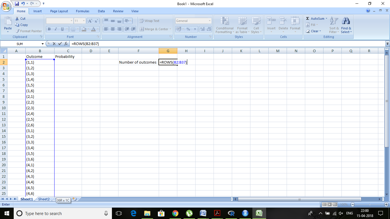
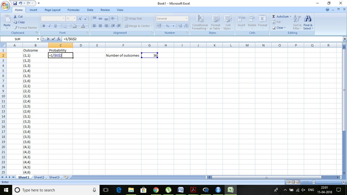
- This will give you total number of outcomes, 36 in our case. Now, in the probability column, select one cell (C2). Type =1/$G$2 in it and then press enter. It gives the decimal value of 1/36. Drag the formula up to the last observation.
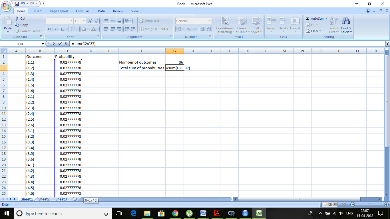
- Now, apply the sum() function to find if the total probability is 1.
- Select both the columns and their observation by ctrl+shift+down and then go to insert>scatter>scatter with only markers.
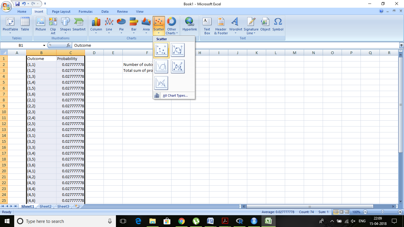
- Set axes labels, title of chart and legend location by going into layout tab. You will get a plot like the following screenshot shows:

You can make the same type of distribution curves with any experiment that produces equally-likely outcomes and have no bias in it. For example, tossing two coins, estimating the likelihood of drawing a particular card from a deck of cards etc. All of these are the examples which generate the uniform probability distributions. Since the data points are discrete in nature, the probability distribution curve will also be discrete.
So, with this we conclude our tutorial. In the next tutorial, we will talk about the concept of expected value, standard deviation, variance and binomial probability distribution. Stay tuned!


