

Linear Regression using Python
Hi MLEnthusiasts! In this tutorial, we will learn how to implement Linear Regression using Python, how to visualize our variables, i.e., do plotting and how to do mathematical computation of R square using Python. Please note that this tutorials is based on our previous tutorial “The Mathematics behind Univariate Linear Regression“. So it is highly recommended to first go through that tutorial to understand this tutorial.
Importing the libraries
The first step is to import Python libraries like NumPy and matplotlib.
import numpy as np
import matplotlib.pyplot as plt
It should be noted over here that np and plt are used as alias names for numpy and matplotlib.pyplot respectively.
Making blank lists
The next step is to make empty vectors for X and Y where X is our input vector and Y is our output vector.
X_input = []           #Making empty list for storing input column
Y_output = []          #Making empty list for storing output column
Opening the data file
Now, we will open our file using the following code:
for line in open("data.csv"): #Reading data.csv line by line
    x, y = line.split(',')     #splitting the line using comma: ","
    X_input.append(float(x)) #Appending the float values of x to empty list
    Y_input.append(float(y)) #Appending the float values of y to empty list
What this will do is it will read the .csv file line by line and will make the observation before ‘,’ get written into x and that after ‘,’ written into y for each line. This will, henceforth, generate two vectors x and y with x being input vector and y being output vector. After this, we will convert the values in x and y into float and will then append those values in X and Y. Therefore, X and Y will also be vectors having values of float data type.
Converting data into NumPy arrays
The next step is to convert X and Y into numpy arrays since numpy makes it very easy to do mathematical computations on its matrices and vectors.
X_input = np.array(X_input)    #Converting X_input list into numpy array
Y_output = np.array(Y_output)  #Converting Y_output list into numpy array
Bivariate analysis using scatter plot
Now, let’s see how the relationship between X and Y looks like.
plt.scatter(X_input, Y_output)
plt.title('Scatter plot showing relationship between X and Y')
plt.xlabel('values of X')
plt.ylabel('values of Y')
plt.show()
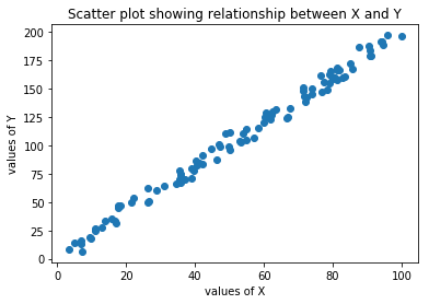
From the above plot, we can see that the relationship is very linear.
Finding co-efficient and intercept
Now, let’s find out what the values of m and c are!
denominator = X_input.dot(X_input) - X_input.mean()*X_input.sum()
m = (X_input.dot(Y_output) - Y_output.mean()*X_input.sum())/denominator  #Slope of linear regression equation
c = (Y_output.mean()*X_input.dot(X_input) - X_input.mean()*X_input.dot(Y_output))/denominator  #Intercept of linear regression equation
print("Value of slope m is", m)
print("Value of intercept c is", c)
Predicting using regression equation
Let’s now find our predicted values for Y or Yhat using linear regression equation.
Yhat = m*X_input + c
Predictions v/s actual values
Let’s visualize how far our predictions are from actual values.
plt.scatter(X_input,Y_output)
plt.title('Scatter plot showing relationship between X and Y')
plt.xlabel('values of X')
plt.ylabel('values of Y')
plt.plot(X_input, Yhat, color = 'red')
plt.show()
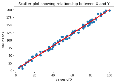
The dots are the actual values of Y and the line of best fit shows Yhat or the predicted values of Y. We see that predictions are very close to the actual values.
Calculating R-square of the model
Let’s now calculate the R square of this model.
diff1 = Y_output - Yhat  #The error term
diff2 = Y_output - Y_output.mean()
rsquared = 1 - (diff1.dot(diff1)/diff2.dot(diff2))
print("R square of the model is", rsquared)
The R square turns out to be very close to 1. Thus our model is very good. It is to be noted here that X.dot(X) = sum of square of Xi where i ranges from 1 to N. N is the number of observations.
So guys, with this, we conclude our tutorial. Stay tuned for more interesting tutorials.


Lovely tutorial, in which you refer to a file data.csv. I’ve read the previous “The Mathematics Behind Univariate Linear Regression”, assuming the file would be referenced in there, but not that I can see. Can you direct me to this file?