

Moore’s Law using Python
Hi All! Today, we will learn how to implement Moore’s Law Using Python using Linear Regression. Before going through this tutorial, it is highly recommended to go through the mathematics behind this tutorial.
What is Moore’s law?
Gordon Moore, the co-founder of Intel proposed Moore’s law in 1965.
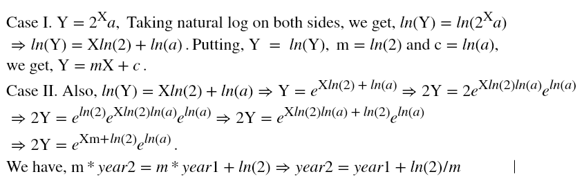
It states that in an Integrated Circuit, the transistor count doubles every year or transistor count, Y = a*2^X where a is any arbitrary constant and X is the time in years.
It also states that though the transistor count gets doubled but the cost of computers gets halved. According to him, we can also expect to see the speed and capacity of computers getting manifolds every few years.
The Code
Below is the implementation of this law using Python.
#importing package for regular expressions
import re
#import numpy to make matrix and vector computations easier
import numpy as np
#import matplotlib.pyplot to visualize the vectors on graphs
import matplotlib.pyplot as plt
#making empty X_input list for the input vector
X_input = []
#making empty Y_output list for the output vector
Y_output = []
#using regular expressions for splitting the data and then substituting it with other values
non_dec = re.compile(r'[^\d]+')
for l in open("moore_law.csv"):
reg = l.split('\t')
x = int(non_dec.sub('', reg[2].split('[')[0]))
y = int(non_dec.sub('', reg[1].split('[')[0]))
X_input.append(x)
Y_output.append(y)
#converting X_input into numpy array
X_input = np.array(X_input)
#converting Y_output into numpy array
Y_output = np.array(Y_output)
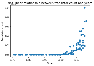
#making scatter plot of X_input and Y_output to see the relationship between them
plt.scatter(X_input, Y_output)
plt.title('Non-linear relationship between transistor count and years')
plt.xlabel('Years')
plt.ylabel('Transistor count')
plt.show()
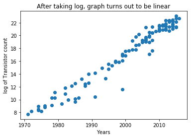
#Since Y_output = a*2^X_input, taking the log of Y_output and then drawing the scatter plot of log(Y_output) and X_input.
Y_output = np.log(Y_output)
plt.scatter(X_input, Y_output)
plt.title('After taking log, graph turns out to be linear')
plt.xlabel('Years')
plt.ylabel('log of Transistor count')
plt.show()
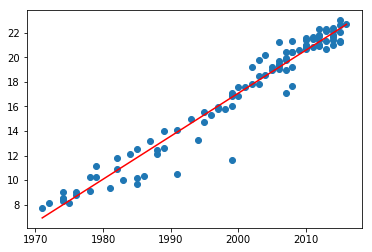
#Calculating m and c and then finding predicted Y or Yhat
denominator = X_input.dot(X_input) - X_input.mean()*X_input.sum()
m = (X_input.dot(Y_output)-Y_output.mean()*X_input.sum())/denominator
c = (Y_output.mean()*X_input.dot(X_input) - X_input.mean()*X_input.dot(Y_output))/denominator
#Calculating Yhat
Yhat = m*X_input + c
plt.scatter(X_input, Y_output)
plt.plot(X_input, Yhat, color='red')
plt.show()
#Calculating Rsquare
diff1 = Y_output - Yhat
diff2 = Y_output - Y_output.mean()
rsquare = 1 - (diff1.dot(diff1)/diff2.dot(diff2))
print("m:", m, "c:", c)
print("The R squared is:", rsquare)
print("time to double is ", np.log(2)/m, "years")
Don’t forget to subscribe to our YouTube channel.


