Ridge Regression Using Python

Hi Everyone! Today, we will learn about ridge regression, the mathematics behind ridge regression and how to implement it using Python!

Foundation for implementation

Sum of squares function

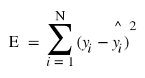
• Firstly, let us have a look at the Sum of square of errors function, that is defined as
• It is also important to note that the first requirement that should be fulfilled for any data set that we want to use for making machine learning models is that the data points should be random in nature and data size should be large.
• But this requirement is not fulfilled sometimes. That is, in some cases, number of features/dimensions(D) is greater than the number of samples/observations(N). Thus, the data set becomes fatty(D >> N) in nature instead of skinny(D << N).
• One thing to be noted is that even completely random noise can also improve R squared. But, this is very unwanted. We don’t want to let noise or unwanted features alter our outputs. This can be achieved by means of regularization.
• In case of L2 regularization, the values of weights are generally kept small, so the affect of noise is generally minimized.

Gaussian distribution and probability

• For any data set which is random in nature, it should follow Gaussian distribution.
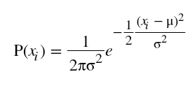
• Any Gaussian distribution is defined by its mean, µ and variance,  and is represented by where X is the input matrix.
• For any point x_i, the probability of x_i is given by the expression.
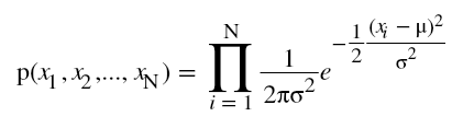
• Also, because the occurrence of each x_i is independent to the occurrence of other, the joint probability of each of them is given by 

• Also, linear regression is the solution which gives the maximum likelihood to the line of best fit.

Likelihood function

• Now, the question arises, what is likelihood? We define likelihood as the probability of data X given a parameter of interest, in our case, it’s µ. So, we write likelihood function as .
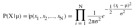• Linear regression maximizes this function for the sake of finding the line of best fit. We do this by finding the value of µ for which this function is maximized and we can say that it is very likely that our data has come from a population that has µ as mean.
• For solving this, first we take the natural log of the likelihood function(L), then differentiate L wrt  µ and then equate this to zero. 

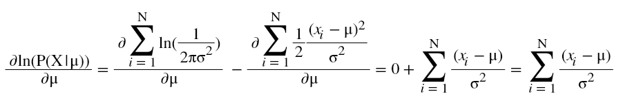
Hence. at this value of µ, the likelihood function is maximized.

• One thing to note here is that maximizing likelihood function L is equivalent to minimizing error function E. Also, y is Gaussian distributed with mean transpose(w)*X and variance sigma-square or or  where ε is Gaussian distributed noise with zero mean and sigma-square variance.
• This is equivalent to saying that in linear regression, errors are Gaussian and the trend is linear.

Why we needed L2 regularization?

• Now, let’s understand why we needed Ridge regression or L2 regularization. The answer is outliers! In the presence of outliers, the linear regression gets the line of best fit diverted from the real trend. This is because it follows the method of least squares and in order to minimize the error, it makes the trend line bent towards the outliers. This makes the prediction less accurate and far from what could be in the absence of outliers. To handle this problem, we needed the method of L2 Regularization or Ridge regression.

Cost function and penalties

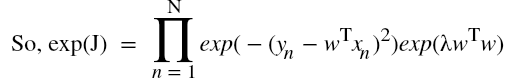
• To compensate for this, we modify the cost function and penalize the large weights in the following way

• Plain squared error maximizes likelihood as shown above. But now, since we have two terms in the cost function, we no longer do this. We now have two probabilities, one is likelihood probability and other one is prior. 
• Note: In the above images, it’s not posterior but it’s likelihood.

• We call P(w) prior because it represents our prior beliefs about w. Thus, now, J is proportional to -ln(P(Y|X, w))-ln(P(w)). Also, by Baye’s rule, we get, P(w|Y,X) is proportional to P(Y|X,w)*P(w). We call P(w|Y,X) as the Posterior probability. We call the method of maximizing P(w|Y,X) as Maximizing A Posterior or MAP.
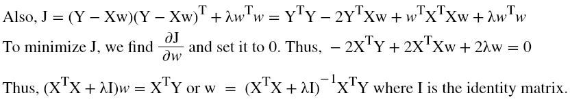
• This method encourages the weights to be small as P(w) is a Gaussian centered around 0. We call the above value of w as the MAP estimate of w.

Implementation of Ridge Regression using Python

Now, let’s see how to implement Ridge regression or L2 regularization in Python.

Importing the libraries

import numpy as np              #importing the numpy package with alias np
import matplotlib.pyplot as plt #importing the matplotlib.pyplot as plt

No_of_observations = 50                         #Setting number of observation = 50

X_input = np.linspace(0,10,No_of_observations)        #Generating 50 equally-spaced data points between 0 to 10.
Y_output = 0.5*X_input + np.random.randn(No_of_observations)   #setting Y_outputi = 0.5X_inputi + some random noise

Y_output[-1]+=30   #setting last element of Y_output as Y_output + 30
Y_output[-2]+=30   #setting second last element of Y_output as Y_output + 30

Visualizing input and output

In [18]:

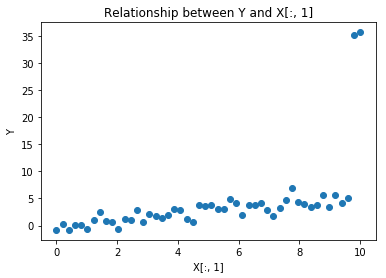
plt.scatter(X_input, Y_output)
plt.title('Relationship between Y and X[:, 1]')
plt.xlabel('X[:, 1]')
plt.ylabel('Y')
plt.show()

X_input = np.vstack([np.ones(No_of_observations), X_input]).T       #appending bias data points colummn to X

w_maxLikelihood = np.linalg.solve(np.dot(X_input.T, X_input), np.dot(X_input.T, Y_output))     #finding weights for maximum likelihood estimation
Y_maxLikelihood = np.dot(X_input, w_maxLikelihood)                                     #Finding predicted Y corresponding to w_ml

Visualizing maximum likelihood function

In [21]:

plt.scatter(X_input[:,1], Y_output)
plt.plot(X_input[:,1],Y_maxLikelihood, color='red')
plt.title('Graph of maximum likelihood method(Red line: predictions)')
plt.xlabel('X[:, 1]')
plt.ylabel('Y')
plt.show()

L2_coeff = 1000    #setting L2 regularization parameter to 1000
w_maxAPosterior = np.linalg.solve(np.dot(X_input.T, X_input)+L2_coeff*np.eye(2), np.dot(X_input.T, Y_output))     #Finding weights for MAP estimation
Y_maxAPosterior = np.dot(X_input, w_maxAPosterior)            #Finding predicted Y corresponding to w_maxAPosterior

MAP v/s Maximum Likelihood

In [28]:

plt.scatter(X_input[:,1], Y_output)
plt.plot(X_input[:,1],Y_maxLikelihood, color='red',label="maximum likelihood")
plt.plot(X_input[:,1],Y_maxAPosterior, color='green', label="map")
plt.title('Graph of MAP v/s ML method')
plt.legend()
plt.xlabel('X[:, 1]')
plt.ylabel('Y')
plt.show()