

Decision Trees using R: An Introduction
Hi MLEnthusiasts! Today, we will dive deeper into classification and will learn about Decision trees using R, how to analyse which variable is important among many given variables and how to make prediction for new data observations based on our analysis and model. Again, we will continue working on the titanic dataset. This will serve our two purposes. One is to learn how to implement classification using decision trees in R and other is by doing this, we will be able to come out with the comparison among the different classification algorithms, which one is better?
Importing the data
So, like always, the first step is to set our working directory and import the dataset.
setwd("C:/Users/jyoti/Desktop/MachineLearning/Classification")
titanicData <- read.csv("titanic.csv")
Summarizing the data
Let’s then find out the summary of this data.
summary(titanicData)## pclass survived name
## Min. :1.00 Min. :0.0000 Connolly, Miss. Kate : 2
## 1st Qu.:2.00 1st Qu.:0.0000 Kelly, Mr. James : 2
## Median :3.00 Median :0.0000 Abbing, Mr. Anthony : 1
## Mean :2.31 Mean :0.3827 Abbott, Master. Eugene Joseph : 1
## 3rd Qu.:3.00 3rd Qu.:1.0000 Abbott, Mr. Rossmore Edward : 1
## Max. :3.00 Max. :1.0000 Abbott, Mrs. Stanton (Rosa Hunt): 1
## (Other) :1249
## sex age sibsp parch
## female:452 Min. : 1.00 Min. :0.000 Min. :0.0000
## male :805 1st Qu.:21.00 1st Qu.:0.000 1st Qu.:0.0000
## Median :28.00 Median :0.000 Median :0.0000
## Mean :29.07 Mean :0.502 Mean :0.3779
## 3rd Qu.:37.00 3rd Qu.:1.000 3rd Qu.:0.0000
## Max. :60.00 Max. :8.000 Max. :9.0000
## NA's :261
## fare embarked
## Min. : 0.000 C:256
## 1st Qu.: 7.896 Q:119
## Median : 14.400 S:882
## Mean : 32.721
## 3rd Qu.: 31.000
## Max. :512.329
##
Using distributions for missing value imputation
As you can see, there are 261 missing values in the age column. Let’s fix that first. Let’s find out the distribution of age variable so that we can understand which value can be used to do missing value imputation.
hist(titanicData$age)
The distribution is more or less normal in nature. Let’s then go ahead with replacing all the missing values by the mean of the age variable. This can be done by using the following R code.
titanicData$age[is.na(titanicData$age)] = 29.07
summary(titanicData)
## pclass survived name
## Min. :1.00 Min. :0.0000 Connolly, Miss. Kate : 2
## 1st Qu.:2.00 1st Qu.:0.0000 Kelly, Mr. James : 2
## Median :3.00 Median :0.0000 Abbing, Mr. Anthony : 1
## Mean :2.31 Mean :0.3827 Abbott, Master. Eugene Joseph : 1
## 3rd Qu.:3.00 3rd Qu.:1.0000 Abbott, Mr. Rossmore Edward : 1
## Max. :3.00 Max. :1.0000 Abbott, Mrs. Stanton (Rosa Hunt): 1
## (Other) :1249
## sex age sibsp parch
## female:452 Min. : 1.00 Min. :0.000 Min. :0.0000
## male :805 1st Qu.:22.00 1st Qu.:0.000 1st Qu.:0.0000
## Median :29.07 Median :0.000 Median :0.0000
## Mean :29.07 Mean :0.502 Mean :0.3779
## 3rd Qu.:34.00 3rd Qu.:1.000 3rd Qu.:0.0000
## Max. :60.00 Max. :8.000 Max. :9.0000
##
## fare embarked
## Min. : 0.000 C:256
## 1st Qu.: 7.896 Q:119
## Median : 14.400 S:882
## Mean : 32.721
## 3rd Qu.: 31.000
## Max. :512.329
## Next step is to view how the dataset looks like.
head(titanicData)## pclass survived name sex
## 1 1 1 Allen, Miss. Elisabeth Walton female
## 2 1 0 Allison, Miss. Helen Loraine female
## 3 1 0 Allison, Mr. Hudson Joshua Creighton male
## 4 1 0 Allison, Mrs. Hudson J C (Bessie Waldo Daniels) female
## 5 1 1 Anderson, Mr. Harry male
## 6 1 0 Andrews, Mr. Thomas Jr male
## age sibsp parch fare embarked
## 1 29 0 0 211.3375 S
## 2 2 1 2 151.5500 S
## 3 30 1 2 151.5500 S
## 4 25 1 2 151.5500 S
## 5 48 0 0 26.5500 S
## 6 39 0 0 0.0000 SUnivariate analysis for obtaining decision trees using R
Let’s do some data manipulation to make the dataset useful for model making.
titanicData$female = ifelse(titanicData$sex=="female", 1, 0)
titanicData$embarked_c = ifelse(titanicData$embarked=="C", 1, 0)
titanicData$embarked_s = ifelse(titanicData$embarked=="S", 1, 0)
titanicData$pclass = as.factor(titanicData$pclass)
titanicData$survived = as.factor(titanicData$survived)
head(titanicData)
## pclass survived name sex
## 1 1 1 Allen, Miss. Elisabeth Walton female
## 2 1 0 Allison, Miss. Helen Loraine female
## 3 1 0 Allison, Mr. Hudson Joshua Creighton male
## 4 1 0 Allison, Mrs. Hudson J C (Bessie Waldo Daniels) female
## 5 1 1 Anderson, Mr. Harry male
## 6 1 0 Andrews, Mr. Thomas Jr male
## age sibsp parch fare embarked female embarked_c embarked_s
## 1 29 0 0 211.3375 S 1 0 1
## 2 2 1 2 151.5500 S 1 0 1
## 3 30 1 2 151.5500 S 0 0 1
## 4 25 1 2 151.5500 S 1 0 1
## 5 48 0 0 26.5500 S 0 0 1
## 6 39 0 0 0.0000 S 0 0 1Removing variables to obtain useful data
Having done that, we also realize that the variables name, sex, embarked are no longer useful to us. So we remove them from our dataframe.
titanicData <- titanicData[-c(3, 4, 9)]Outlier manipulation
Let’s now see if the numerical variables like age and fare have expected quantiles or that also needs manipulation.
bx = boxplot(titanicData$age)
As you can see there are outliers which need to be handled.
bx$stats## [,1]
## [1,] 4.00
## [2,] 22.00
## [3,] 29.07
## [4,] 34.00
## [5,] 52.00quantile(titanicData$age, seq(0, 1, 0.02))## 0% 2% 4% 6% 8% 10% 12% 14% 16%
## 1.0000 3.0000 7.0000 11.0000 15.0000 17.0000 18.0000 18.0000 19.0000
## 18% 20% 22% 24% 26% 28% 30% 32% 34%
## 20.0000 21.0000 21.3200 22.0000 23.0000 24.0000 24.0000 25.0000 25.0000
## 36% 38% 40% 42% 44% 46% 48% 50% 52%
## 26.0000 27.0000 28.0000 29.0000 29.0448 29.0700 29.0700 29.0700 29.0700
## 54% 56% 58% 60% 62% 64% 66% 68% 70%
## 29.0700 29.0700 29.0700 29.0700 29.0700 29.0700 30.0000 30.5000 32.0000
## 72% 74% 76% 78% 80% 82% 84% 86% 88%
## 32.5000 34.0000 35.0000 36.0000 37.0000 39.0000 40.0000 42.0000 44.0000
## 90% 92% 94% 96% 98% 100%
## 45.0000 47.0000 50.0000 52.0000 55.4400 60.0000titanicData$age = ifelse(titanicData$age >= 52, 52, titanicData$age)
titanicData$age = ifelse(titanicData$age <= 4, 4, titanicData$age)
boxplot(titanicData$age)
Perfect! Let’s do the same for fare variable.
bx = boxplot(titanicData$fare)
bx$stats## [,1]
## [1,] 0.0000
## [2,] 7.8958
## [3,] 14.4000
## [4,] 31.0000
## [5,] 65.0000quantile(titanicData$fare, seq(0, 1, 0.02))## 0% 2% 4% 6% 8% 10%
## 0.000000 6.495800 7.125000 7.229200 7.250000 7.550000
## 12% 14% 16% 18% 20% 22%
## 7.740524 7.750000 7.750000 7.775000 7.854200 7.879200
## 24% 26% 28% 30% 32% 34%
## 7.895800 7.895800 7.925000 8.050000 8.050000 8.662500
## 36% 38% 40% 42% 44% 46%
## 9.034672 9.838676 10.500000 11.760000 13.000000 13.000000
## 48% 50% 52% 54% 56% 58%
## 13.000000 14.400000 15.045800 15.550000 16.100000 20.212500
## 60% 62% 64% 66% 68% 70%
## 21.045000 23.250000 25.895672 26.000000 26.020000 26.550000
## 72% 74% 76% 78% 80% 82%
## 27.900000 30.000000 31.387500 36.350000 39.687500 50.456136
## 84% 86% 88% 90% 92% 94%
## 53.176000 59.400000 69.550000 76.952520 83.158300 108.009000
## 96% 98% 100%
## 136.504184 211.500000 512.329200To avoid data loss, let’s limit the significance level to 96%.
titanicData$fare = ifelse(titanicData$fare >= 136, 136, titanicData$fare)
boxplot(titanicData$fare)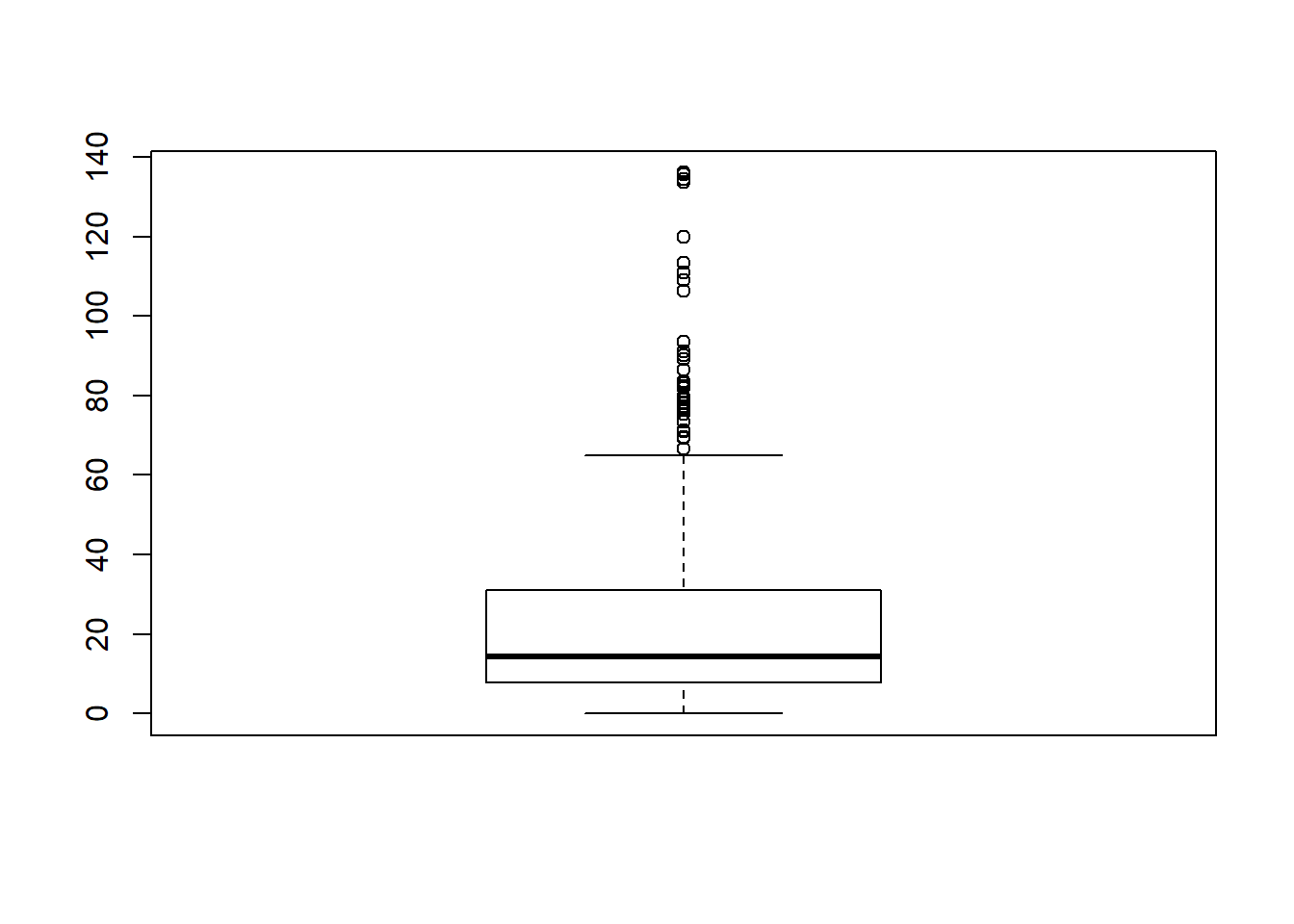
Let’s now start the bivariate analysis of our dataset. First let’s do the boxplot analysis of survived with age and survived with fare.
boxplot(titanicData$age~titanicData$survived, main="Boxplot for age variable")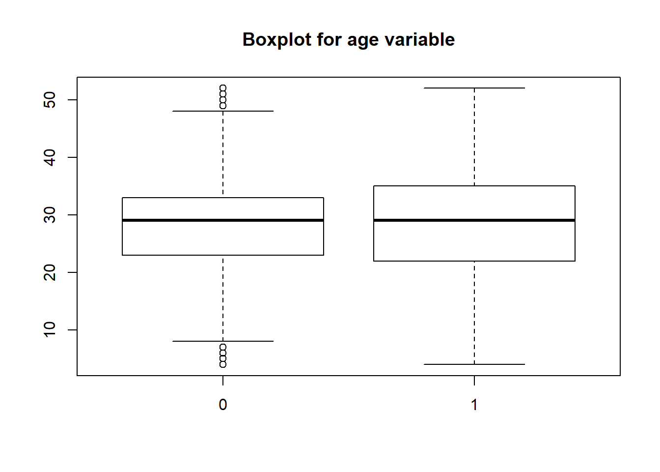
It looks like people who died were mainly of middle age as the whiskers for 0 start at 10 and end at 48 approximately.
boxplot(titanicData$fare~titanicData$survived, main="Boxplot for fare variable")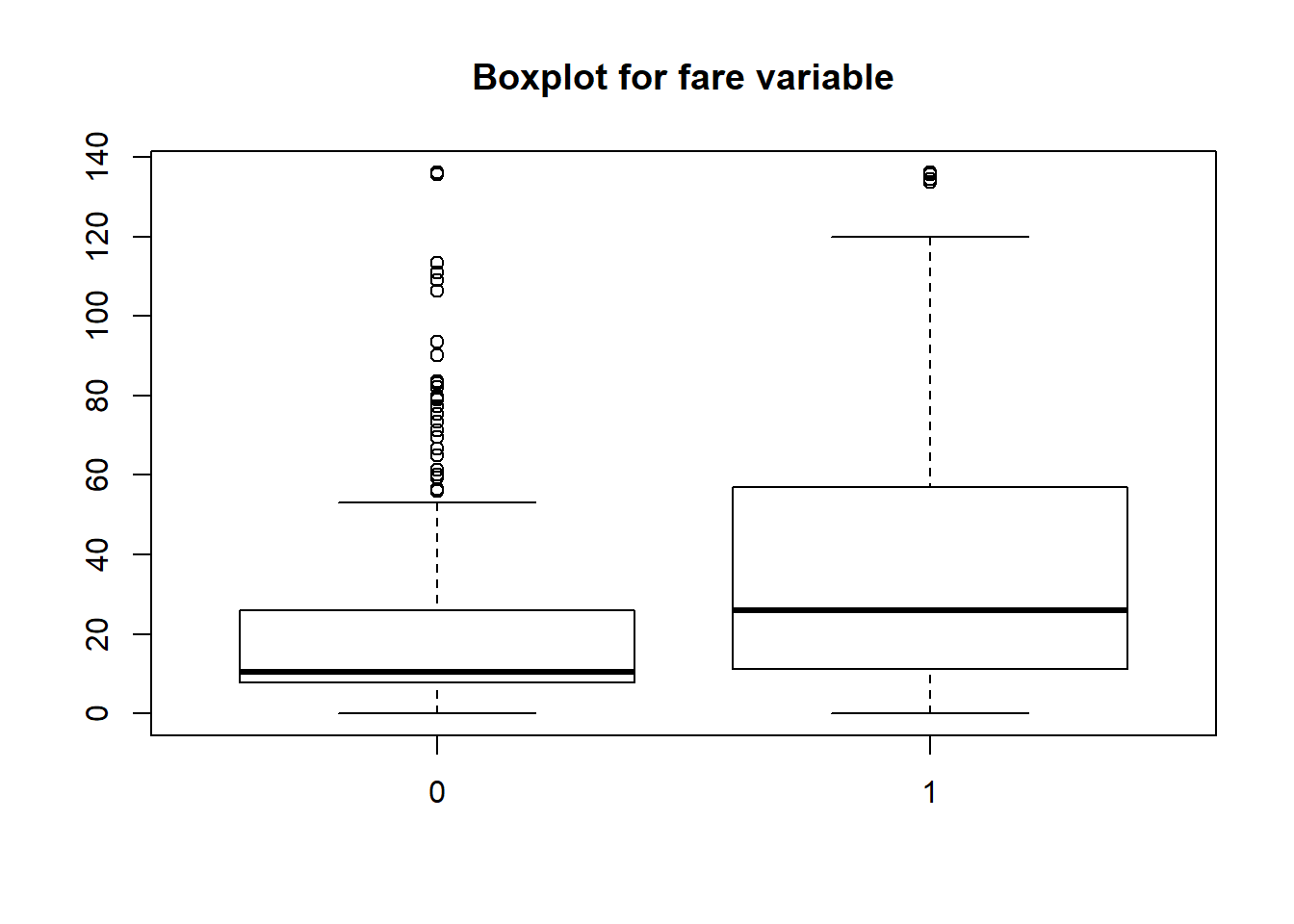
It looks like people who died had also some relation with fare! Those who died had paid lower(though there are outliers too). Those who survived had paid comparatively higher fare.
Bivariate analysis for obtaining decision trees using R
For categorical variables, we will do bivariate analysis using mosaic plot.
mosaicplot(titanicData$pclass~titanicData$survived, main="Boxplot for pclass variable", color="skyblue")
This indeed reveals a useful trend. 1. People of 1st class had a better survival rate among all the classes. 2. People of 3sr class had the worst survival rate.
mosaicplot(titanicData$female~titanicData$survived, main="Boxplot for gender vs survival analysis", color="skyblue")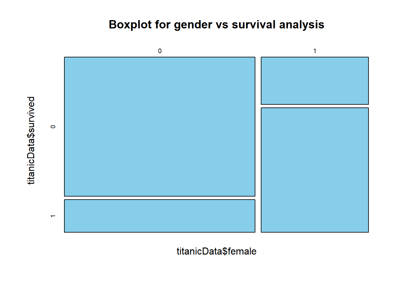
Male passengers had worse survival rate than the females. It seems like females were saved first when the mishap happened.
mosaicplot(titanicData$embarked_c~titanicData$survived, main="Boxplot for embarkment as C variable", color="skyblue")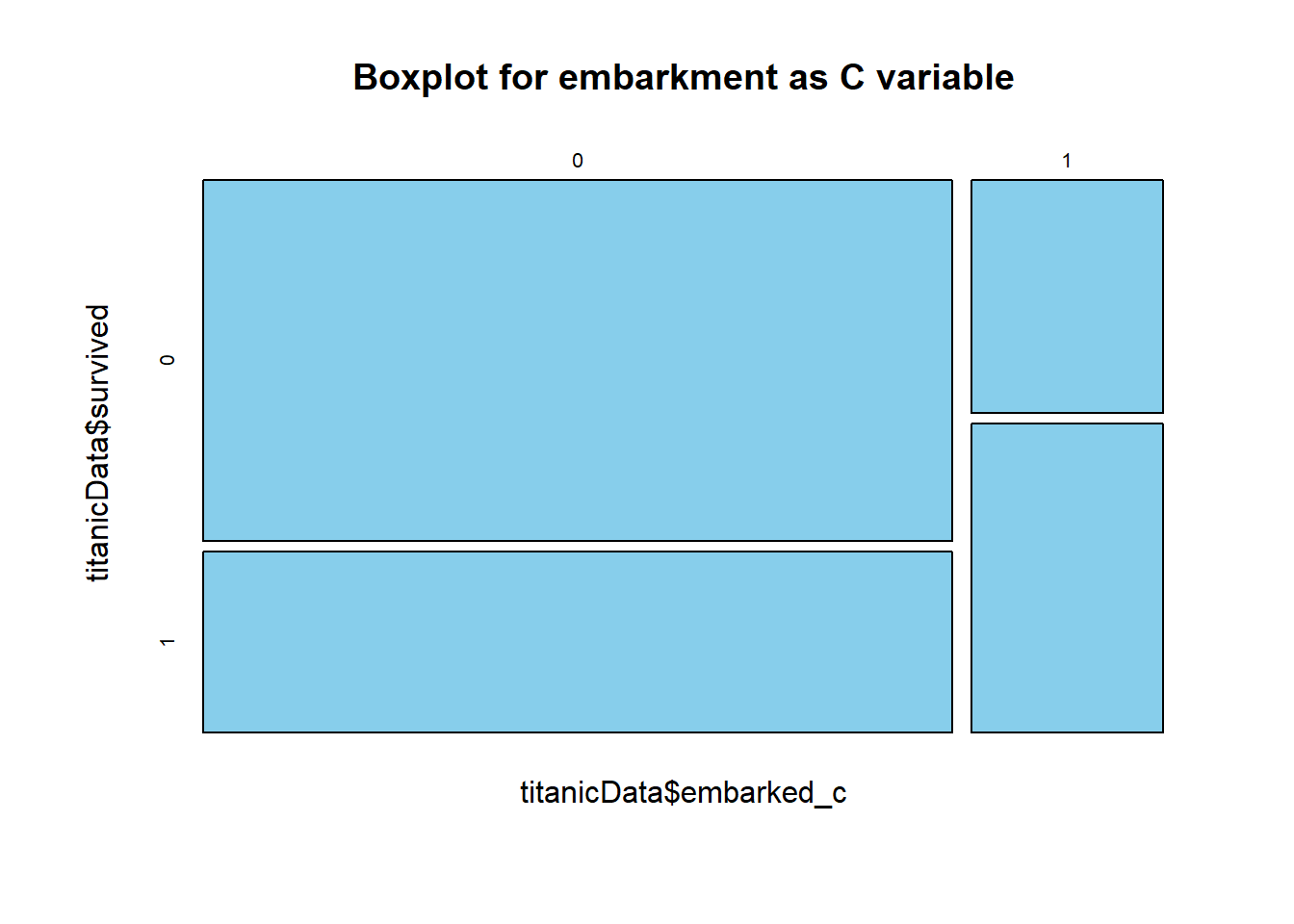
From the chart, it looks like the survival rate for the embarkment other than port “C” is worse than port “C”.
mosaicplot(titanicData$embarked_s~titanicData$survived, main="Boxplot for embarkment as S variable", color="skyblue")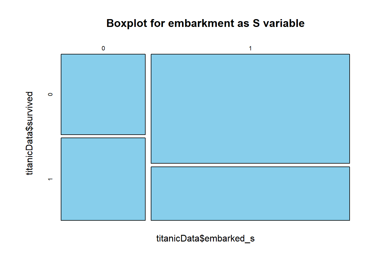
We can see from the chart that the survival rate for port “S” was very very good, far better than the other two ports.
Correlation Analysis
Let’s now do the correlation analysis of the above data. As the cor() function takes only numerical data, let’s first convert all the categorical columns into numerical and store it into new dataframe.
titanicDataNumerical = data.frame(titanicData)
titanicDataNumerical$pclass = as.numeric(titanicData$pclass)
titanicDataNumerical$survived = as.numeric(titanicData$survived)
titanicDataNumerical$sibsp = as.numeric(titanicData$sibsp)
titanicDataNumerical$parch = as.numeric(titanicData$parch)
titanicDataNumerical$female = as.numeric(titanicData$female)
titanicDataNumerical$embarked_c = as.numeric(titanicData$embarked_c)
titanicDataNumerical$embarked_s = as.numeric(titanicData$embarked_s)
titanicDataNumerical$age = titanicData$age
titanicDataNumerical$fare = titanicData$fare
Now, let’s find the correlation among all of them.
library(corrplot)## corrplot 0.84 loadedcor(titanicDataNumerical)## pclass survived age sibsp parch
## pclass 1.00000000 -0.32725083 -0.35309876 0.06180422 0.02620263
## survived -0.32725083 1.00000000 -0.01493079 -0.03480143 0.07444689
## age -0.35309876 -0.01493079 1.00000000 -0.20017298 -0.12191168
## sibsp 0.06180422 -0.03480143 -0.20017298 1.00000000 0.37679176
## parch 0.02620263 0.07444689 -0.12191168 0.37679176 1.00000000
## fare -0.67866086 0.29736533 0.18218451 0.22825539 0.24633570
## female -0.13406341 0.52881727 -0.04420916 0.10218247 0.22136893
## embarked_c -0.28849436 0.19525216 0.09624283 -0.05332157 -0.01313978
## embarked_s 0.10529179 -0.16636744 -0.06024244 0.07613393 0.07398385
## fare female embarked_c embarked_s
## pclass -0.6786609 -0.13406341 -0.28849436 0.10529179
## survived 0.2973653 0.52881727 0.19525216 -0.16636744
## age 0.1821845 -0.04420916 0.09624283 -0.06024244
## sibsp 0.2282554 0.10218247 -0.05332157 0.07613393
## parch 0.2463357 0.22136893 -0.01313978 0.07398385
## fare 1.0000000 0.22875075 0.31638709 -0.17604836
## female 0.2287507 1.00000000 0.06564176 -0.12013483
## embarked_c 0.3163871 0.06564176 1.00000000 -0.77557107
## embarked_s -0.1760484 -0.12013483 -0.77557107 1.00000000corrplot(cor(titanicDataNumerical), method="circle")
So, we can say that survival is mainly related to age, pclass, fare, female, embarked_c and embarked_S.
Splitting the data for training and testing the model
Let’s do the splitting of dataset between training and test sets.
set.seed(1234)
split = sample(1:nrow(titanicData), 0.7*nrow(titanicData))
trainSplit = titanicData[split, ]
testSplit = titanicData[-split,]
print(table(trainSplit$survived))
##
## 0 1
## 527 352print(table(testSplit$survived))##
## 0 1
## 249 129Now let’s check for event rate.
prop.table(table(trainSplit$survived))##
## 0 1
## 0.5995449 0.4004551prop.table(table(testSplit$survived))##
## 0 1
## 0.6587302 0.3412698So, the probabilities are approx same in both train and test datasets.
Modeling decision trees using R
We can now start building our decision tree using rpart algorithm.
library(rpart)
library(rpart.plot)
fit = rpart(survived~., data=trainSplit, method="class", control=rpart.control(minsplit=10, cp=0.008))
rpart.plot(fit)
Thus, total 13 nodes get created in this case. Each node shows: 1. the predicted class(0 for not survived, 1 for survived) 2. predicted probability of survival 3. The percentage of observations in each of the node.
summary(fit)## Call:
## rpart(formula = survived ~ ., data = trainSplit, method = "class",
## control = rpart.control(minsplit = 10, cp = 0.008))
## n= 879
##
## CP nsplit rel error xerror xstd
## 1 0.451704545 0 1.0000000 1.0000000 0.04127048
## 2 0.022727273 1 0.5482955 0.5482955 0.03486612
## 3 0.009943182 3 0.5028409 0.5284091 0.03440218
## 4 0.008049242 6 0.4715909 0.5539773 0.03499518
## 5 0.008000000 12 0.4232955 0.5511364 0.03493084
##
## Variable importance
## female fare pclass age parch sibsp
## 44 20 15 8 7 4
## embarked_c embarked_s
## 1 1
##
## Node number 1: 879 observations, complexity param=0.4517045
## predicted class=0 expected loss=0.4004551 P(node) =1
## class counts: 527 352
## probabilities: 0.600 0.400
## left son=2 (558 obs) right son=3 (321 obs)
## Primary splits:
## female < 0.5 to the left, improve=121.91870, (0 missing)
## fare < 50.7396 to the left, improve= 37.66640, (0 missing)
## pclass splits as RLL, improve= 34.90510, (0 missing)
## embarked_c < 0.5 to the left, improve= 17.17411, (0 missing)
## embarked_s < 0.5 to the right, improve= 11.27987, (0 missing)
## Surrogate splits:
## parch < 0.5 to the left, agree=0.675, adj=0.109, (0 split)
## fare < 75.7667 to the left, agree=0.675, adj=0.109, (0 split)
## age < 9.5 to the right, agree=0.644, adj=0.025, (0 split)
##
## Node number 2: 558 observations, complexity param=0.008049242
## predicted class=0 expected loss=0.2007168 P(node) =0.6348123
## class counts: 446 112
## probabilities: 0.799 0.201
## left son=4 (451 obs) right son=5 (107 obs)
## Primary splits:
## pclass splits as RLL, improve=7.934882, (0 missing)
## fare < 26.26875 to the left, improve=5.945697, (0 missing)
## embarked_c < 0.5 to the left, improve=5.110501, (0 missing)
## age < 13.5 to the right, improve=4.484881, (0 missing)
## embarked_s < 0.5 to the right, improve=2.662998, (0 missing)
## Surrogate splits:
## fare < 26.26875 to the left, agree=0.889, adj=0.421, (0 split)
## age < 44.5 to the left, agree=0.841, adj=0.168, (0 split)
##
## Node number 3: 321 observations, complexity param=0.02272727
## predicted class=1 expected loss=0.2523364 P(node) =0.3651877
## class counts: 81 240
## probabilities: 0.252 0.748
## left son=6 (145 obs) right son=7 (176 obs)
## Primary splits:
## pclass splits as RRL, improve=29.788890, (0 missing)
## fare < 48.2021 to the left, improve=12.223650, (0 missing)
## embarked_c < 0.5 to the left, improve= 7.004200, (0 missing)
## sibsp < 2.5 to the right, improve= 4.677233, (0 missing)
## parch < 3.5 to the right, improve= 4.063987, (0 missing)
## Surrogate splits:
## fare < 22.67915 to the left, agree=0.819, adj=0.600, (0 split)
## age < 29.535 to the left, agree=0.667, adj=0.262, (0 split)
## sibsp < 1.5 to the right, agree=0.579, adj=0.069, (0 split)
## parch < 2.5 to the right, agree=0.567, adj=0.041, (0 split)
## embarked_c < 0.5 to the left, agree=0.555, adj=0.014, (0 split)
##
## Node number 4: 451 observations, complexity param=0.008049242
## predicted class=0 expected loss=0.1596452 P(node) =0.513083
## class counts: 379 72
## probabilities: 0.840 0.160
## left son=8 (430 obs) right son=9 (21 obs)
## Primary splits:
## age < 9.5 to the right, improve=4.4139660, (0 missing)
## parch < 0.5 to the left, improve=0.9013663, (0 missing)
## embarked_c < 0.5 to the left, improve=0.7373491, (0 missing)
## fare < 51.6979 to the left, improve=0.6388989, (0 missing)
## sibsp < 3.5 to the right, improve=0.3591483, (0 missing)
## Surrogate splits:
## sibsp < 2.5 to the left, agree=0.956, adj=0.048, (0 split)
##
## Node number 5: 107 observations, complexity param=0.008049242
## predicted class=0 expected loss=0.3738318 P(node) =0.1217292
## class counts: 67 40
## probabilities: 0.626 0.374
## left son=10 (104 obs) right son=11 (3 obs)
## Primary splits:
## age < 15 to the right, improve=2.4203810, (0 missing)
## embarked_c < 0.5 to the left, improve=2.3709840, (0 missing)
## embarked_s < 0.5 to the right, improve=2.0337560, (0 missing)
## parch < 1.5 to the left, improve=1.0909330, (0 missing)
## fare < 109.8916 to the left, improve=0.8876608, (0 missing)
##
## Node number 6: 145 observations, complexity param=0.02272727
## predicted class=1 expected loss=0.4896552 P(node) =0.1649602
## class counts: 71 74
## probabilities: 0.490 0.510
## left son=12 (20 obs) right son=13 (125 obs)
## Primary splits:
## fare < 23.35 to the right, improve=7.812966, (0 missing)
## embarked_s < 0.5 to the right, improve=3.617690, (0 missing)
## embarked_c < 0.5 to the left, improve=3.407144, (0 missing)
## parch < 1.5 to the right, improve=2.780228, (0 missing)
## sibsp < 2.5 to the right, improve=2.232369, (0 missing)
## Surrogate splits:
## sibsp < 2.5 to the right, agree=0.897, adj=0.25, (0 split)
## parch < 1.5 to the right, agree=0.897, adj=0.25, (0 split)
##
## Node number 7: 176 observations
## predicted class=1 expected loss=0.05681818 P(node) =0.2002275
## class counts: 10 166
## probabilities: 0.057 0.943
##
## Node number 8: 430 observations
## predicted class=0 expected loss=0.144186 P(node) =0.4891923
## class counts: 368 62
## probabilities: 0.856 0.144
##
## Node number 9: 21 observations, complexity param=0.008049242
## predicted class=0 expected loss=0.4761905 P(node) =0.02389078
## class counts: 11 10
## probabilities: 0.524 0.476
## left son=18 (11 obs) right son=19 (10 obs)
## Primary splits:
## sibsp < 2.5 to the right, improve=6.8580090, (0 missing)
## pclass splits as -RL, improve=3.6011900, (0 missing)
## fare < 19.9125 to the right, improve=2.1428570, (0 missing)
## embarked_s < 0.5 to the left, improve=1.0011900, (0 missing)
## age < 7.5 to the left, improve=0.7408964, (0 missing)
## Surrogate splits:
## fare < 19.9125 to the right, agree=0.810, adj=0.6, (0 split)
## pclass splits as -RL, agree=0.762, adj=0.5, (0 split)
## age < 5.5 to the left, agree=0.619, adj=0.2, (0 split)
## parch < 1.5 to the right, agree=0.619, adj=0.2, (0 split)
## embarked_c < 0.5 to the left, agree=0.619, adj=0.2, (0 split)
##
## Node number 10: 104 observations, complexity param=0.008049242
## predicted class=0 expected loss=0.3557692 P(node) =0.1183163
## class counts: 67 37
## probabilities: 0.644 0.356
## left son=20 (67 obs) right son=21 (37 obs)
## Primary splits:
## embarked_c < 0.5 to the left, improve=1.9627100, (0 missing)
## embarked_s < 0.5 to the right, improve=1.6651020, (0 missing)
## fare < 58.575 to the right, improve=1.2640680, (0 missing)
## age < 49.5 to the right, improve=0.7287281, (0 missing)
## sibsp < 0.5 to the left, improve=0.2355769, (0 missing)
## Surrogate splits:
## embarked_s < 0.5 to the right, agree=0.990, adj=0.973, (0 split)
## fare < 53.99795 to the left, agree=0.692, adj=0.135, (0 split)
## age < 50.5 to the left, agree=0.663, adj=0.054, (0 split)
##
## Node number 11: 3 observations
## predicted class=1 expected loss=0 P(node) =0.003412969
## class counts: 0 3
## probabilities: 0.000 1.000
##
## Node number 12: 20 observations
## predicted class=0 expected loss=0.1 P(node) =0.02275313
## class counts: 18 2
## probabilities: 0.900 0.100
##
## Node number 13: 125 observations, complexity param=0.009943182
## predicted class=1 expected loss=0.424 P(node) =0.1422071
## class counts: 53 72
## probabilities: 0.424 0.576
## left son=26 (97 obs) right son=27 (28 obs)
## Primary splits:
## fare < 15.3729 to the left, improve=2.1848660, (0 missing)
## embarked_c < 0.5 to the left, improve=2.0420970, (0 missing)
## age < 29.535 to the right, improve=1.9308760, (0 missing)
## embarked_s < 0.5 to the right, improve=1.1204990, (0 missing)
## parch < 0.5 to the left, improve=0.2686984, (0 missing)
## Surrogate splits:
## parch < 2.5 to the left, agree=0.792, adj=0.071, (0 split)
## age < 8.5 to the right, agree=0.784, adj=0.036, (0 split)
## sibsp < 1.5 to the left, agree=0.784, adj=0.036, (0 split)
##
## Node number 18: 11 observations
## predicted class=0 expected loss=0.09090909 P(node) =0.01251422
## class counts: 10 1
## probabilities: 0.909 0.091
##
## Node number 19: 10 observations
## predicted class=1 expected loss=0.1 P(node) =0.01137656
## class counts: 1 9
## probabilities: 0.100 0.900
##
## Node number 20: 67 observations
## predicted class=0 expected loss=0.2835821 P(node) =0.07622298
## class counts: 48 19
## probabilities: 0.716 0.284
##
## Node number 21: 37 observations, complexity param=0.008049242
## predicted class=0 expected loss=0.4864865 P(node) =0.04209329
## class counts: 19 18
## probabilities: 0.514 0.486
## left son=42 (17 obs) right son=43 (20 obs)
## Primary splits:
## fare < 58.575 to the right, improve=2.327663000, (0 missing)
## age < 49.5 to the right, improve=1.430542000, (0 missing)
## sibsp < 0.5 to the left, improve=0.008225617, (0 missing)
## parch < 0.5 to the left, improve=0.003727866, (0 missing)
## Surrogate splits:
## parch < 0.5 to the right, agree=0.757, adj=0.471, (0 split)
## sibsp < 0.5 to the right, agree=0.703, adj=0.353, (0 split)
## age < 32.25 to the right, agree=0.649, adj=0.235, (0 split)
##
## Node number 26: 97 observations, complexity param=0.009943182
## predicted class=1 expected loss=0.4742268 P(node) =0.1103527
## class counts: 46 51
## probabilities: 0.474 0.526
## left son=52 (53 obs) right son=53 (44 obs)
## Primary splits:
## age < 23.5 to the right, improve=1.9697620, (0 missing)
## fare < 7.26665 to the right, improve=1.6568480, (0 missing)
## embarked_c < 0.5 to the left, improve=0.8326725, (0 missing)
## parch < 1.5 to the right, improve=0.4736981, (0 missing)
## embarked_s < 0.5 to the right, improve=0.2722423, (0 missing)
## Surrogate splits:
## fare < 7.9771 to the left, agree=0.608, adj=0.136, (0 split)
## sibsp < 0.5 to the left, agree=0.588, adj=0.091, (0 split)
## parch < 0.5 to the left, agree=0.577, adj=0.068, (0 split)
## embarked_s < 0.5 to the left, agree=0.577, adj=0.068, (0 split)
## embarked_c < 0.5 to the left, agree=0.557, adj=0.023, (0 split)
##
## Node number 27: 28 observations
## predicted class=1 expected loss=0.25 P(node) =0.03185438
## class counts: 7 21
## probabilities: 0.250 0.750
##
## Node number 42: 17 observations
## predicted class=0 expected loss=0.2941176 P(node) =0.01934016
## class counts: 12 5
## probabilities: 0.706 0.294
##
## Node number 43: 20 observations
## predicted class=1 expected loss=0.35 P(node) =0.02275313
## class counts: 7 13
## probabilities: 0.350 0.650
##
## Node number 52: 53 observations, complexity param=0.009943182
## predicted class=0 expected loss=0.4339623 P(node) =0.06029579
## class counts: 30 23
## probabilities: 0.566 0.434
## left son=104 (49 obs) right son=105 (4 obs)
## Primary splits:
## fare < 7.3896 to the right, improve=2.7724300, (0 missing)
## embarked_s < 0.5 to the right, improve=0.8883106, (0 missing)
## sibsp < 0.5 to the right, improve=0.6377358, (0 missing)
## parch < 0.5 to the right, improve=0.6377358, (0 missing)
## age < 29.535 to the right, improve=0.4237008, (0 missing)
##
## Node number 53: 44 observations
## predicted class=1 expected loss=0.3636364 P(node) =0.05005688
## class counts: 16 28
## probabilities: 0.364 0.636
##
## Node number 104: 49 observations
## predicted class=0 expected loss=0.3877551 P(node) =0.05574516
## class counts: 30 19
## probabilities: 0.612 0.388
##
## Node number 105: 4 observations
## predicted class=1 expected loss=0 P(node) =0.004550626
## class counts: 0 4
## probabilities: 0.000 1.000CP is the complexity parameter. It prevents overfitting and controls the size of the tree. To get added into a node, a variable has to be having CP less than 0.008 or else tree building will not continue.
print(fit)## n= 879
##
## node), split, n, loss, yval, (yprob)
## * denotes terminal node
##
## 1) root 879 352 0 (0.59954494 0.40045506)
## 2) female< 0.5 558 112 0 (0.79928315 0.20071685) ## 4) pclass=2,3 451 72 0 (0.84035477 0.15964523) ## 8) age>=9.5 430 62 0 (0.85581395 0.14418605) *
## 9) age< 9.5 21 10 0 (0.52380952 0.47619048) ## 18) sibsp>=2.5 11 1 0 (0.90909091 0.09090909) *
## 19) sibsp< 2.5 10 1 1 (0.10000000 0.90000000) * ## 5) pclass=1 107 40 0 (0.62616822 0.37383178) ## 10) age>=15 104 37 0 (0.64423077 0.35576923)
## 20) embarked_c< 0.5 67 19 0 (0.71641791 0.28358209) * ## 21) embarked_c>=0.5 37 18 0 (0.51351351 0.48648649)
## 42) fare>=58.575 17 5 0 (0.70588235 0.29411765) *
## 43) fare< 58.575 20 7 1 (0.35000000 0.65000000) *
## 11) age< 15 3 0 1 (0.00000000 1.00000000) * ## 3) female>=0.5 321 81 1 (0.25233645 0.74766355)
## 6) pclass=3 145 71 1 (0.48965517 0.51034483)
## 12) fare>=23.35 20 2 0 (0.90000000 0.10000000) *
## 13) fare< 23.35 125 53 1 (0.42400000 0.57600000)
## 26) fare< 15.3729 97 46 1 (0.47422680 0.52577320) ## 52) age>=23.5 53 23 0 (0.56603774 0.43396226)
## 104) fare>=7.3896 49 19 0 (0.61224490 0.38775510) *
## 105) fare< 7.3896 4 0 1 (0.00000000 1.00000000) *
## 53) age< 23.5 44 16 1 (0.36363636 0.63636364) * ## 27) fare>=15.3729 28 7 1 (0.25000000 0.75000000) *
## 7) pclass=1,2 176 10 1 (0.05681818 0.94318182) *prp(fit)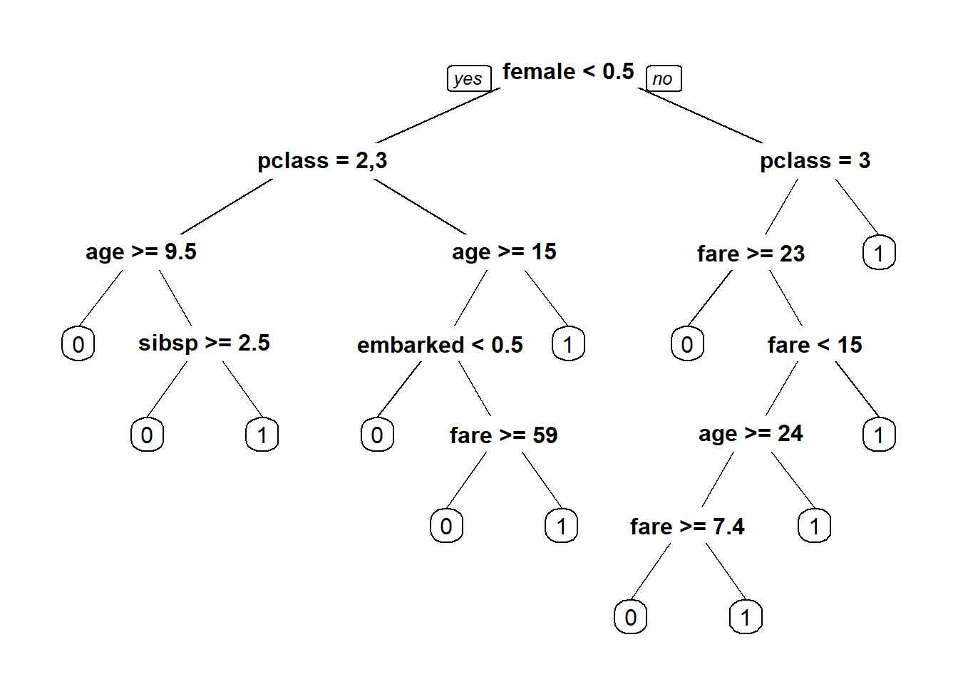
There are 6 leaf nodes representing class 0 and 7 leaf nodes representing class 1. Now, let’s plot CP values.
plotcp(fit)
printcp(fit)##
## Classification tree:
## rpart(formula = survived ~ ., data = trainSplit, method = "class",
## control = rpart.control(minsplit = 10, cp = 0.008))
##
## Variables actually used in tree construction:
## [1] age embarked_c fare female pclass sibsp
##
## Root node error: 352/879 = 0.40046
##
## n= 879
##
## CP nsplit rel error xerror xstd
## 1 0.4517045 0 1.00000 1.00000 0.041270
## 2 0.0227273 1 0.54830 0.54830 0.034866
## 3 0.0099432 3 0.50284 0.52841 0.034402
## 4 0.0080492 6 0.47159 0.55398 0.034995
## 5 0.0080000 12 0.42330 0.55114 0.034931Predicting by decision trees using R
Now, let’s make the predictions.
predictTrain = predict(fit, trainSplit, type="class")
table(predictTrain, trainSplit$survived)
##
## predictTrain 0 1
## 0 486 108
## 1 41 244Thus, Accuracy for training dataset = 730/879 = 83.05%.
predictTest = predict(fit, testSplit, type = "class")
table(predictTest, testSplit$survived)
##
## predictTest 0 1
## 0 223 44
## 1 26 85Thus, Accuracy for test dataset = 308/378 = 81.48%. As compared to the logistic regression, which gives the accuracy of 80% on the training dataset and 78.83% on test dataset, decision tree gives the accuracy of 83.05% on the training dataset and 81.5% on the test dataset.


Excellent explanation Jyoti for the beginners. Thanks for sharing.Keep it up. I am your big fan as you explain the procesd so simply. Can you please write blog on Bagging, Boosting and XGBOOST.
Hi Ash! I thank you for this appreciation. People like you give a boost to us to work harder. All our hard work gets paid off when we see that our posts are able to help the beginners in their mission.
I will surely write on the topics that you have mentioned over here. 🙂
Excellent presentation U Rockk