

Adjusted Returns including Inflation
Hi All! In the part 6 of Financial Analytics series, we learnt how to fetch historical financial data from multiple sources using Python. In this tutorial, we will learn the ways of considering inflation in a return series to obtain adjusted returns including inflation and implementing them using Python. We will be fetching data from quandl and yfinance in this tutorial, so I recommend you to read part 6 of Financial Analytics series first. Also, if you’re new to this series and want to learn Financial Analytics using Python, go to part 1 of Financial Analytics series to have a good head-start!
Adjusted Returns including Inflation – Formula
We have R’ = (1 + R)/(1 + I) – 1
Here, R = simple return series, I = inflation rate series, R’ = Return series with inflation
Step 1: Downloading Customer Price Index from Quandl
# Importing libraries
import pandas as pd
import quandl as qd
import yfinance as yf
key = 'key_comes_here'
#Key authentication - key to be fetched from https://www.quandl.com/account/profile after signing up
qd.ApiConfig.api_key = key
#Fetching CPI - Customer Price Index for USA from quandl
USA_CPI = qd.get(dataset='RATEINF/CPI_USA',
                  start_date='2008-04-01',
                  end_date='2018-03-31')
#Checking head of the dataframe
USA_CPI.head()
# Renaming Value column to CPI
# Calling rename function on USA_CPI and passing dictionary to columns having keys as old column names and values as new column names
USA_CPI.rename(columns = {'Value': 'CPI'}, inplace = True)
USA_CPI.head()
Step 2: Fetching stocks data from yfinance
# Downloading MSFT data from yfinance from 1st April 2008 to 31st March 2018
msftStockData = yf.download( 'MSFT',
                        start = '2008-04-01',
                        end = '2018-03-31',
                        progress = False)
# Checking what's in there the dataframe by loading first 5 rows
msftStockData.head()
Step 3: Making a date dataframe
dates = pd.DataFrame(index=pd.date_range(start='2008-04-01',
                                         end='2018-03-31'))
dates.head()
Step 4: Joining dates and stock data
# Joining by calling join function on dates dataframe.
# In how parameter, we specify which join we want to perform
# how = 'left' performs left join in which all rows of dates are fetched and matching rows from msftStockData is returned
# Unmatched values have NaN or Not a Number
# We are only interested in Adjusted close column, so we will include only that column from the right table
Date_Stock = dates.join(msftStockData[['Adj Close']], how = 'left')
Date_Stock.head(10)
# In order to handling missing values, let's use missing value imputation
# Importing simpleImputer class from sklearn.impute library
from sklearn.impute import SimpleImputer

#Inititalizing the object of SimpleImputer class
data_Imputer = SimpleImputer()

#Fitting and transforming the data using the data_Imputer object and then wrapping it around pd.DataFrame function to convert it into a dataframe from numpy array.
imputedData = pd.DataFrame(data_Imputer.fit_transform(Date_Stock))
imputedData.head(10)
# Replacing values from imputedData to Adj Close column of Date_Stock
Date_Stock['Adj Close'] = imputedData[0].values
Date_Stock.head(10)
# Selecting end of month rows only to do Month on Month analysis
Date_Stock = Date_Stock.asfreq('M')
Date_Stock.head(10)
Step 5: Joining Stock and CPI data
# Left joining stock and USA inflation (Customer Price Index) data
Stock_Inflation = Date_Stock.join(USA_CPI, how = 'left')
Stock_Inflation.head()
Step 6: Calculating simple returns and inflation rate
#Calculating simple returns by pct_change() function of the dataframe
Stock_Inflation['Simple Return'] = Stock_Inflation['Adj Close'].pct_change()
Stock_Inflation.head()
#Calculating inflation rate by pct_change() function of the dataframe
Stock_Inflation['Inflation rate'] = Stock_Inflation['CPI'].pct_change()
Stock_Inflation.head()
Step 7: Considering inflation rate in returns
# Applying the formula R' = (1 + Simple Return)/(1 + Inflation rate) - 1
Stock_Inflation['Adj Return'] = ((1 + Stock_Inflation['Simple Return'])/(1 + Stock_Inflation['Inflation rate'])) - 1
Stock_Inflation.head()
Step 8: Seeing the results on line charts
# importing matplotlib library
import matplotlib.pyplot as plt
# Seeing simple return on line chart
Stock_Inflation['Simple Return'].plot(figsize = (14,10))

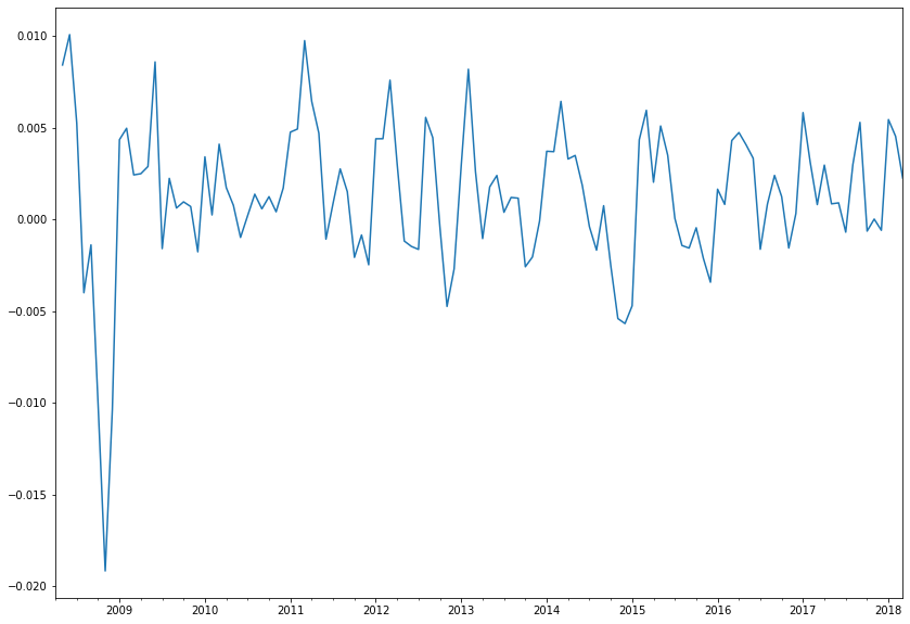
# Seeing adjusted return on line chart
Stock_Inflation['Adj Return'].plot(figsize = (14,10))

# Seeing inflation rate on line chart
Stock_Inflation['Inflation rate'].plot(figsize = (14,10))
So guys, in this tutorial, we learnt how to obtain adjusted return – considering inflation rate in simple returns.
Stay tuned for next tutorial on this Financial Analytics series. Don’t forget to subscribe to our YouTube channel.


One thought on “Adjusted Returns including Inflation: FA7”