The Perceptron: A theoretical Approach

Hi ML Enthusiasts! Today, we will take the first step towards learning Artificial Neural Networks. In this post, we will learn about the functioning of neural networks and their analogy with human brain and neurons.

For learning how to implement the perceptron algorithm using python, please go through our this post on How to implement the perceptron algorithm using Python.

The Brain and The Neurons

Human brain is the best example of learning by experience. The concept of generalizing by past experience, adapting to new changes and making decisions based on memories are best seen in the human brain. So, let’s learn about the basic working of brain and neurons.

• Neurons are the basic processing units of the brain.
• Transmitter chemicals are present within the fluid of the brain. These chemicals work in such a way that they raise or lower down the electric potential of the neuron.
• If this potential exceeds a pre-defined threshold, the neuron spikes, else it doesn’t. The spike is nothing but a pulse of fixed strength and duration that is sent to axon.
• This axon divides into further connections to other neurons.
• After spiking/firing, a neuron has to wait for a fixed amount of time to regain its energy and momentum back.
• There is a concept of plasticity which corresponds to modifying the strength of synaptic connections(connection between axons of multiple neurons) to make the system adaptable.

Thus, one can say that a neuron is a processor/computer. With so many neurons in the brain, the brain is a hub to so many processors/computers.

To increase our understanding of the neural networks, let’s learn about Hebb’s rule first.

Hebb’s Rule

Hebb’s rule helps us in understanding that the relation between strength of synaptic connections and firing of these two connecting neurons. Thus, if there are any changes in the strength of synaptic connections, then these changes are proportional to the correlation in the firing of these connecting neurons. Thus, if two neurons fire simultaneously, the connection between them increases in strength. If they never fire simultaneously, the strength of their connection decreases.

McCulloch and Pitts Neurons

McCulloch and Pitts modelled a neurons as:

• The synapses inputs were modelled as a set of weighted inputs w_i.
• The inputs x_i‘s correspond to the input nodes.
• The transfer function/adder which adds up these weighted inputs that corresponds to the potential that the chemical produces.
• An activation function that correspond to the threshold function that decides whether the neuron fires or not.

To understand more about it, please have a look at the picture shown below:

Here, i represents the number of input nodes and j represents the number of output nodes. If there are n neurons, then there will be n output nodes each corresponding to one neuron. Also, there will be m input nodes for each neuron. The weighted inputs are nothing but the inputs at the input nodes get multiplied with the weights in the circle. These weights represent the strength of the synapses. Higher the weight, higher the effect of input at that particular node. The weighted inputs get added(transfer function) and the net input gets compared with the threshold value. Depending on whether it exceeds the threshold value or not, it fires or doesn’t fire thus producing output at the output node.

Thus, for each neuron j, the transfer function becomes

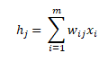
Also, the output for each output node j is given by the following equation:

where θ is the value given by threshold function.

• Outputs: The model will predict some output o_j. Here, j varies from 1 to n.
• Targets: The target variable is the actual output values which we will provide to the model for the purpose of supervised learning. The algorithm will use these target values of the training data to learn by means of algorithm. They contain the correct answers to every observation. We will use t_j to represent target/actual output of every output node.
• Error: The error e_j corresponds to the difference between o_j and t_j or

The Approach

The idea is that firstly, we choose any random values of the weights and then apply inputs x_i to the input nodes. Using these random weights, the first prediction is made. The prediction is subtracted from the corresponding target observations to produce errors. These errors are then used to make the weights adaptable using the following equations:

Here, η is called as the learning rate.

The Learning Rate

The learning rate tells the algorithm how much to change the weights by. Very less value of learning rate will make the algorithm run slower than desired. But, it will also make the algorithm more stable and resistant to any inaccuracies. Very large value will make the algorithm never reach the optimum value. Thus, learning rate should be chosen very carefully. Usually, 0.1 ≤ η ≤ 0.4 is the moderate interval for choosing the value of learning rate.

The Bias Input

In order to make the threshold adaptable to any changes, so that neuron firing is made adaptable, we use the bias node. Let’s consider a situation where all the inputs are zero. Now, it doesn’t matter what the weights are since all the inputs are zero. So, to make the neuron fire, we need to adjust the threshold value. If we need to fix the threshold at zero, we include a bias node having input as -1 and we can choose any random weight. Since, the weights are adaptable, the weight to the bias node also gets changed. The only thing impacting the output and weights is the bias node in this case. Bias input node is represented by x₀ and the bias weight is represented by w_0j.

The Perceptron Algorithm

The perceptron algorithm is divided into three phases:

• Initialization phase : In this phase, we set the weights to any random values. They can be positive or negative.
• Training phase: 
  • For T iterations
    • For each input vector
      • Forward Propagation: Compute the activation and predicted outputs using the following equations:

 Backward Propagation: Update the weights using the following equation:

• Recall Phase: Compute the activation of the neuron j using the final weights using the following equations:

Please note that for training phase, the time complexity is O(Tmn) because it involves T iterations and for recall phase, the time complexity is O(mn).

So guys, with this we conclude our tutorial. Stay tuned for more interesting blog posts.