

Hi MLEnthusiasts! In the last tutorial, we had learnt about the basics of clustering and its types. In this tutorial, we will learn about the theory behind K-means clustering and its optimization. It is recommended to go through Clustering-Part 1 tutorial before proceeding with this tutorial.
What is K-means clustering?
K-Means clustering is a type of unsupervised machine learning technique. It involves grouping the unlabeled data based on their similarities and their Euclidean distances. Here, “K” in K-Means Clustering represents the number of groups/clusters. In this algorithm, based on the number of features and feature similarity, each observation is iteratively assigned to one of the K clusters.
It is a partitioning clustering technique the prime objective of which is to maximize the inter-cluster distances and minimize the intra-cluster distances.
Steps involved in carrying out K-Means Clustering
- First select the value of K.
- Randomly choose the initial data-points for all these K clusters. Then put other data-points on the basis of distances between the initial data-points and them.
- Calculate the centroid of all these clusters. A centroid is the mean of all the points in a cluster. Then measure the Euclidean distance of each data-point from each centroid. Put the data point in that cluster the centroid of which has the least distance from the data-point. Run the algorithm for all the data-points. This leads to the formation of K clusters and all the data-points end up in one of these K clusters. This also leads to an initial-clustering.
- Now, re-run the algorithm iteratively till we get the best cluster similarity metrics.
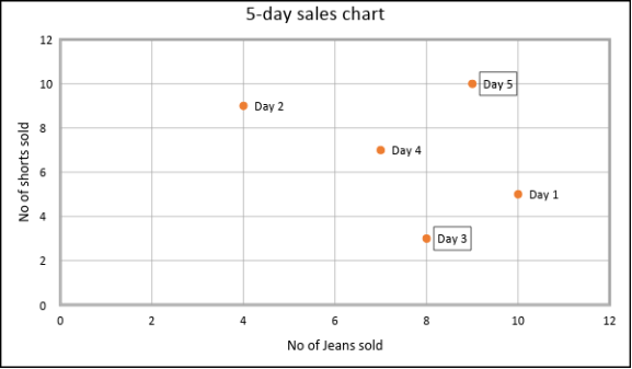
Let’s take an example to understand this. Look at the following table which has the sales data of jeans and shirts for 5 days.
| Sales | No of jeans sold | No of shirts sold |
| Day 1 | 10 | 5 |
| Day 2 | 4 | 9 |
| Day 3 | 8 | 3 |
| Day 4 | 7 | 7 |
| Day 5 | 9 | 10 |
Step 1: Choose the value of K or number of clusters. Let’s take K = 2.
Step 2: Let’s take day 3 and day 5 as initial reference points or centroid
Therefore, C1: (8, 3) and C2: (9, 10)
The formula for calculating the Euclidean distance between two points (x, y) and (a, b) is [(x-a)^2+(y-b)^2]^0.5
Using this formula, we calculate the distance between C1 and each of the other data -points and same we do for C2. We obtain the following table after doing this.
| Sales | Distance from C1 | Distance from C2 | |
| Day 1 | 2.8 | 5.1 | Cluster 1 |
| Day 2 | 7.2 | 5.1 | Cluster 2 |
| Day 3 | 0 | 7.07 | Centroid 1, Cluster 1 |
| Day 4 | 4.1 | 3.6 | Cluster 2 |
| Day 5 | 7.07 | 0 | Centroid 2, Cluster 2 |
From the table, we can say that day 1 and day 3 lie in cluster 1. Day 2, day 4 and day 5 lie in cluster 2.
| Sales | No of jeans sold | No of shirts sold | Cluster |
| Day 1 | 10 | 5 | 1 |
| Day 2 | 4 | 9 | 2 |
| Day 3 | 8 | 3 | 1 |
| Day 4 | 7 | 7 | 2 |
| Day 5 | 9 | 10 | 2 |
This is called as initial-partitioning. Let’s now move to step 3.
Step 3: Calculating the centroids.
Formula: (x, y): (∑xi/n, ∑yi/n) where n is the number of points in a cluster.
Centroid for cluster 1 = (10+8)/2, (5+3)/2= (9, 4) and for cluster 2 = (4+7+9)/3, (9+7+10)/3= (6.7, 8.7).
Now, the centroid for both the clusters have changed.
Step 4: By keeping these points as reference, we again calculate the distance between these centroids and all the data-points. A table similar to that given above is obtained. And then depending upon the distances, we again put them in different clusters. This process is repeated till the algorithm converges.
How to choose the value of K?
The most important step of clustering is also to find that value of K for which the intra-clustering distance or Within cluster Sum of Square (WSS) distance is minimized. This actually tells us how good our clustering is and how compact the clusters are. There are three methods which are used to find out the value of K. They are:
-
Elbow method
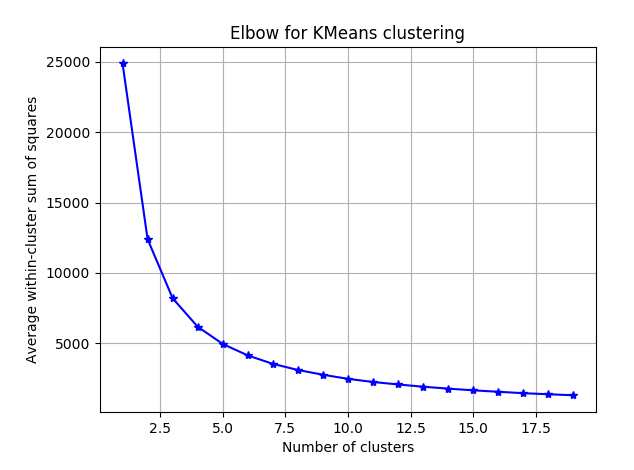
In elbow method, total WSS is measured as a function of K(number of clusters) and this function is plotted to chart with total WSS on the y-axis and values of K on x-axis. The idea is to choose that value of K which falls on the elbow of the curve or to look for that value of K in the graph after which the graph doesn’t show much variation. As the number of clusters, K increases, total WSS decreases with it being equal to zero for K equal to number of data-points. But, it is not optimal to choose that large number of K. Thus, optimal value of K is given by the elbow of this curve.
In the below image, we can choose the optimal value of K to be 5 or 6.
-
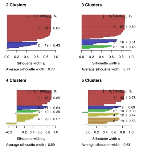
Average Silhouette method
We can determine the quality of clustering using Average Silhouette method. It gives us an idea of how well each data-point of a cluster resides into it. More is the value of average silhouette width, the better is the clustering. So, choose K for which the average Silhouette width metric is the highest. This can also be visualized in a graph which has average Silhouette of observations of the y-axis and number of clusters, K on x-axis. The value of K which has the highest value of average Silhouette of observations is the optimal number of clusters.
Step 1: Choose a value of K.
Step 2: Find the Silhouette co-efficient for each cluster among the K clusters. Silhouette co-efficient for a single cluster among K clusters is given by the following formula:
Si=1-xi/yi or Si=(yi-xi)/max(xi,yi)
where for an individual point i in a particular cluster say cluster A, xi represents the average distance of that point I from other points in the same cluster, i.e., cluster A and yi represents the average distance of point i from other points residing in clusters other than cluster A. This gives the Silhouette co-efficient for every cluster among the K clusters. Generally, Si lies between 0 and 1 with Si closer to 1 indicating good quality of clustering.
Step 3: Find the average Silhouette width(average of all the Si). If it is closer to 1, then it indicates excellent quality of clustering. If it is closer to 0, that means the quality of clustering is not so good.
-
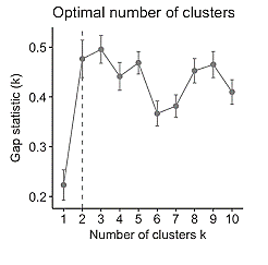
Gap Statistics method
The gap statistic compares the total within intra-cluster variation for different values of k with their expected values under null reference distribution of the data, i.e. a distribution with no obvious clustering. The optimal cluster value will be that smallest value of K which satisfies the following equation:
Gap(K)≥Gap(K+1)-sK+1
Where sK+1 is the 1-standard error at point K+1.
So, in this post, we learnt about the theory behind K-means clustering and different methods which we can use to find out the optimal value of K. In the coming posts, we will cover more about clustering. Till then, stay tuned!


