

Data cleaning – Introduction
While doing data data analysis, before analyzing the data for any kind of resultant, we most perform the most essential step, that is, Data Cleaning. Because when we get the data it may not be ready for complete analysis, like there might me missing values which will make our judgement wrong, outliers which may affect the Mean, Median; variable may spread across the values of a column (need to convert that column into multiple variables. i.e., columns) and many more. So before performing any kind of analysis for getting results by using any means like Linear Regression, we must do data cleaning for getting the accurate results.
Working on dataset for data cleaning
Let’s use one of the data-sets being provided in RStudio, that is, “SURVEY” for data cleaning purposes. It consists of variables like “Age”, “Pulse rate”, “Gender(Sex)”, etc.
library(MASS)
View(survey)
head(survey, 10)
## Sex Wr.Hnd NW.Hnd W.Hnd Fold Pulse Clap Exer Smoke Height
## 1 Female 18.5 18.0 Right R on L 92 Left Some Never 173.00
## 2 Male 19.5 20.5 Left R on L 104 Left None Regul 177.80
## 3 Male 18.0 13.3 Right L on R 87 Neither None Occas NA
## 4 Male 18.8 18.9 Right R on L NA Neither None Never 160.00
## 5 Male 20.0 20.0 Right Neither 35 Right Some Never 165.00
## 6 Female 18.0 17.7 Right L on R 64 Right Some Never 172.72
## 7 Male 17.7 17.7 Right L on R 83 Right Freq Never 182.88
## 8 Female 17.0 17.3 Right R on L 74 Right Freq Never 157.00
## 9 Male 20.0 19.5 Right R on L 72 Right Some Never 175.00
## 10 Male 18.5 18.5 Right R on L 90 Right Some Never 167.00
## M.I Age
## 1 Metric 18.250
## 2 Imperial 17.583
## 3 16.917
## 4 Metric 20.333
## 5 Metric 23.667
## 6 Imperial 21.000
## 7 Imperial 18.833
## 8 Metric 35.833
## 9 Metric 19.000
## 10 Metric 22.333summary(survey)## Sex Wr.Hnd NW.Hnd W.Hnd Fold
## Female:118 Min. :13.00 Min. :12.50 Left : 18 L on R : 99
## Male :118 1st Qu.:17.50 1st Qu.:17.50 Right:218 Neither: 18
## NA's : 1 Median :18.50 Median :18.50 NA's : 1 R on L :120
## Mean :18.67 Mean :18.58
## 3rd Qu.:19.80 3rd Qu.:19.73
## Max. :23.20 Max. :23.50
## NA's :1 NA's :1
## Pulse Clap Exer Smoke Height
## Min. : 35.00 Left : 39 Freq:115 Heavy: 11 Min. :150.0
## 1st Qu.: 66.00 Neither: 50 None: 24 Never:189 1st Qu.:165.0
## Median : 72.50 Right :147 Some: 98 Occas: 19 Median :171.0
## Mean : 74.15 NA's : 1 Regul: 17 Mean :172.4
## 3rd Qu.: 80.00 NA's : 1 3rd Qu.:180.0
## Max. :104.00 Max. :200.0
## NA's :45 NA's :28
## M.I Age
## Imperial: 68 Min. :16.75
## Metric :141 1st Qu.:17.67
## NA's : 28 Median :18.58
## Mean :20.37
## 3rd Qu.:20.17
## Max. :73.00
##
Description of data-set is as follows:
Sex <- The sex of the student (Factor with levels “Male” and “Female”.)
Wr.Hnd <- span (distance from tip of thumb to tip of little finger of spread hand) of writing hand, in centimetres.
NW.Hnd <- span of non-writing hand
W.Hnd <- writing hand of student (Factor, with levels “Left” and “Right”.)
Fold <- Fold your arms! Which is on top (Factor, with levels “R on L”, “L on R”, “Neither”.)
Pulse <- pulse rate of student (beats per minute)
Clap <- Clap your hands! Which hand is on top (Factor, with levels “Right”, “Left”, “Neither”.)
Exer <- how often the student exercises (Factor, with levels “Freq” (frequently), “Some”, “None”.)
Smoke <- how much the student smokes (Factor, levels “Heavy”, “Regul” (regularly), “Occas” (occasionally), “Never”.)
Height <- height of the student in centimetres
M.I. <- whether the student expressed height in imperial (feet/inches) or metric (centimetres/metres) units. (Factor, levels “Metric”, “Imperial”.)
Age <- age of the student in years
By “View()” method above the data set opens separately in RStudio for better view and we can see the data type as well of each variable by hovering onto it.
By “summary()” we got the summary of data like “Min value”, “Max value”, “Mean”, “Frequency”, etc.
The main things that can be interpreted from above summary are:
- Categorical Variables: Sex, W.Hnd, Fold, Clap, Exer, Smoke, M.I
- Numerical Variables: Wr.Hnd, NW.Hnd, Pulse, Height, Age
- Presence of “NA” –> which means that our data-set contains missing or undefined values. While visualising the data using View() we can verify that there are a lot of missing values.
- Other factors like –> Frequecny in case of categorical variable and for Numeric variables we get Mean, Median, Min, Max, 1st and 3rd Quartile.
?? Now the first question would have aroused in your mind that if the data is missing then how we can do proper analysis of data. You would be thinking how we can rplace all “NA” with some data. For that we generally use Mean, Median and Mode.
Filling Up Missing Values:
Since we have worked upon the outliers now we can work upon the missing values. For removing the gaps in information we can replace “NA” with either “Mean”, “Median” or “Mode”, depending upon the scenarios.
Scenarios for Raplcaing Missing Values:
- If variable is “Continuous” –> Replace NA with any either “Mean”, “Median” or “Mode”.
- Otherwise
- If data “Normally Distributed” –> Replace NA with “Mean”.
- if data “Skewd” –> Replace NA with “Median”.
- If “Categorical” –> Replace NA with “Mode”.
** For “Non-continuous Numerical” data we will be using “Histogram” to check distribution of data (Normal or Skewd).
Working on Survey Data-Set:
- For variable “Sex” It is a Categorical variable so we will use Mode.
survey$Sex[is.na(survey$Sex)] <- "Female"
summary(survey$Sex)
## Female Male
## 119 118- For variable “Wr.Hnd” It is a Non-continuous Numerical Variable so first we will look for distribution of data, by using histogram.
hist(survey$Wr.Hnd, main="Wr.Hnd")
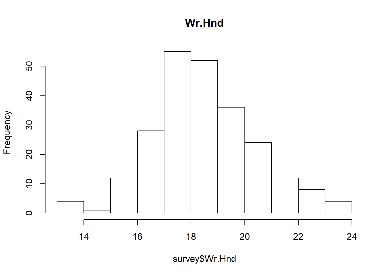
In above histogram we can see that the data is Right-Skewd, so we will replace “NA” with “Median”
survey$Wr.Hnd[is.na(survey$Wr.Hnd)] <- median(survey$Wr.Hnd, na.rm=TRUE)
summary(survey$Wr.Hnd)
## Min. 1st Qu. Median Mean 3rd Qu. Max.
## 13.00 17.50 18.50 18.67 19.80 23.20- For variable “NW.Hnd” It is a Non-continuous Numerical Variable so first we will look for distribution of data, by using histogram.
hist(survey$NW.Hnd, main="NW.Hnd")
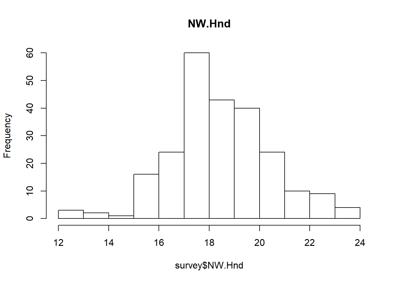
In above histogram we can see that the data is approximately “Right Skewd”, so we will replace “NA” with “Median”
survey$NW.Hnd[is.na(survey$NW.Hnd)] <- median(survey$NW.Hnd, na.rm=TRUE)
summary(survey$NW.Hnd)
## Min. 1st Qu. Median Mean 3rd Qu. Max.
## 12.50 17.50 18.50 18.58 19.70 23.50- For variable “W.Hnd” It is a Categorical variable so we will use Mode.
survey$W.Hnd[is.na(survey$W.Hnd)] <- "Right"
summary(survey$W.Hnd)
## Left Right
## 18 219- For variable “Pulse” It is a Non-continuous Numerical Variable so first we will look for distribution of data, by using histogram.
hist(survey$Pulse, main="Pulse")
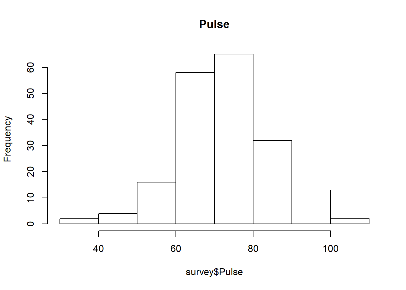
In above histogram we can see that the data is approximately “Normally Distributed”, so we will replace “NA” with “Mean”
survey$Pulse[is.na(survey$Pulse)] <- mean(survey$Pulse, na.rm=TRUE)
summary(survey$Pulse)
## Min. 1st Qu. Median Mean 3rd Qu. Max.
## 35.00 68.00 74.15 74.15 80.00 104.00- For variable “Clap” It is a Categorical variable so we will use Mode.
survey$Clap[is.na(survey$Clap)] <- "Right"
summary(survey$Clap)
## Left Neither Right
## 39 50 148- For variable “Smoke” It is a Categorical variable so we will use Mode.
survey$Smoke[is.na(survey$Smoke)] <- "Never"
summary(survey$Smoke)
## Heavy Never Occas Regul
## 11 190 19 17- For variable “Height” It is a Non-continuous Numerical Variable so first we will look for distribution of data, by using histogram.
hist(survey$Height, main="Height")
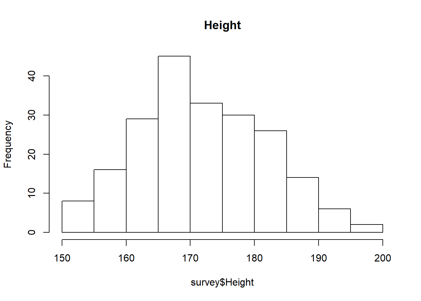
In above histogram we can see that the data is approximately “Right Skewd”, so we will replace “NA” with “median”
survey$Height[is.na(survey$Height)] <- median(survey$Height, na.rm=TRUE)
summary(survey$Height)
## Min. 1st Qu. Median Mean 3rd Qu. Max.
## 150.0 167.0 171.0 172.2 179.0 200.0- For variable “M.I” It is a Categorical variable so we will use Mode.
survey$M.I[is.na(survey$M.I)] <- "Metric"
summary(survey$M.I)
## Imperial Metric
## 68 169summary(survey)## Sex Wr.Hnd NW.Hnd W.Hnd Fold
## Female:119 Min. :13.00 Min. :12.50 Left : 18 L on R : 99
## Male :118 1st Qu.:17.50 1st Qu.:17.50 Right:219 Neither: 18
## Median :18.50 Median :18.50 R on L :120
## Mean :18.67 Mean :18.58
## 3rd Qu.:19.80 3rd Qu.:19.70
## Max. :23.20 Max. :23.50
## Pulse Clap Exer Smoke Height
## Min. : 35.00 Left : 39 Freq:115 Heavy: 11 Min. :150.0
## 1st Qu.: 68.00 Neither: 50 None: 24 Never:190 1st Qu.:167.0
## Median : 74.15 Right :148 Some: 98 Occas: 19 Median :171.0
## Mean : 74.15 Regul: 17 Mean :172.2
## 3rd Qu.: 80.00 3rd Qu.:179.0
## Max. :104.00 Max. :200.0
## M.I Age
## Imperial: 68 Min. :16.75
## Metric :169 1st Qu.:17.67
## Median :18.58
## Mean :20.37
## 3rd Qu.:20.17
## Max. :73.00By following the above process we raplaced all the missing values with some meaningful data, as you can see in the “summary()” of data there are no “NA”s. Now our data is much cleaner than the one we started with, and it looks good for further analysis. Now the next thing that we need to handle is “Outlier”
Outliers
Outliers are the data values which deviate a lot from most of the data values, either too big or too small in comparison to average values. Let us understand using an example…We will use “boxplot()” for finding the outliers.
#We will create it only for numeric variables not for categorical data
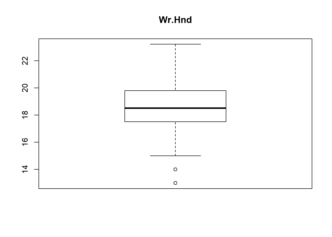
boxplot(survey$Wr.Hnd, main="Wr.Hnd")
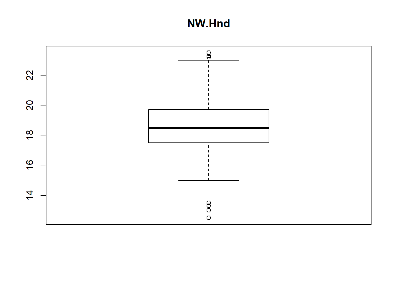
boxplot(survey$NW.Hnd, main="NW.Hnd")
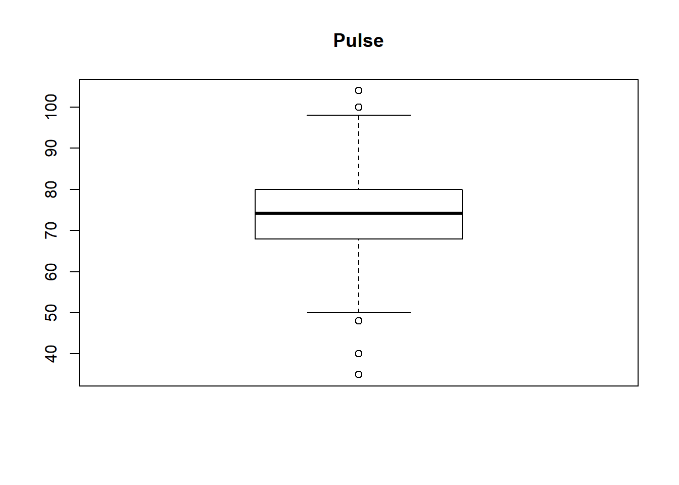
boxplot(survey$Pulse, main="Pulse")
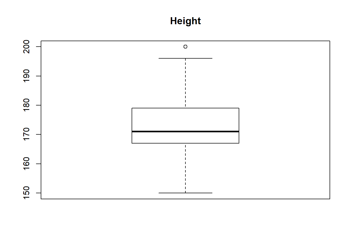
boxplot(survey$Height, main="Height")
boxplot(survey$Age, main="Age")
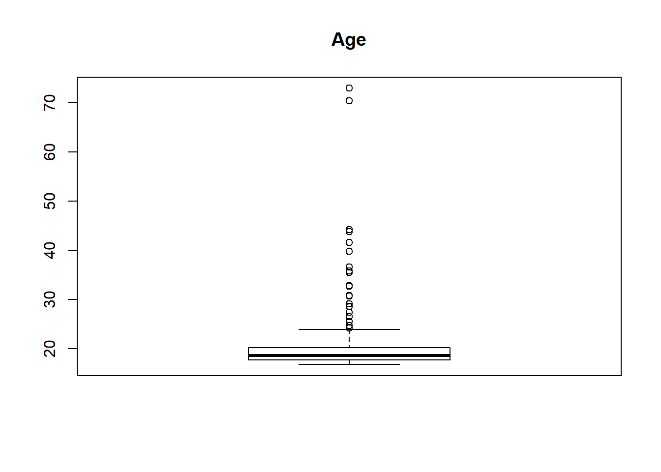
From above boxplot of “survey” data-set we can see that for variables Wr.Hnd, NW.Hnd, Pulse and Age has got some dots or circles in the graph, either above or below the slim lines (called whiskers, 1st and 3rd Quartile of boxplot). Those circles represents the presence of outliers and number of outliers OR we can detect outliers in one more way, that is, all the values out of range of 5th and 95th percentile can be considered as Outlier.
Removing Outliers
We will use the second method for removing the outliers, because in case of boxplot we may endup loosing some crucial information too, as range being produced by the 1st and 3rd quartile is generally smaller in comparison to the range being produced by 5th and 95th percentile. For example:
- Range generated by Quartiles
#For variable PULSE
## Range generated by Quartiles
## (-1.5 * IQR) to (1.5 * IQR), where (Inerquartile Range) IQR <- Q3 -Q1
#Q1 and Q3 are present in summary of Pulse, that we obtained at the beginning

Q3 <- 80
Q1 <- 66
IQR <- Q3 -Q1
lower <- -1.5 * IQR
upper <- 1.5 * IQR

lower
## [1] -21upper## [1] 21- Range generated by 5th and 95th Percentiles
## Range generated by 5th and 95th Percentiles
## For this we use quantile(, ) method

lower <- quantile(survey$Pulse, 0.05, na.rm=TRUE)
upper <- quantile(survey$Pulse, 0.95, na.rm=TRUE)

lower
## 5%
## 60upper## 95%
## 92So we can see the significant difference in the range of values. Thus we will be useing Percentile approach for capping the outliers. ** Another thing to be noted is that in case of Percentiles we are using level of significance, so per our requirement we can change it too. In general we use 5th and 95th percentiles.
After detecting outliers for a variable we will replace it with the Mean of the data. We will do the same procedure for all the variables containing outliers.
- For variable Pulse
quantile(survey$Pulse, 0.05, na.rm=TRUE)## 5%
## 60quantile(survey$Pulse, 0.95, na.rm=TRUE)## 95%
## 92survey$Pulse <- ifelse(survey$Pulse > 92, 74.22, survey$Pulse)
survey$Pulse <- ifelse(survey$Pulse < 60, 74.22, survey$Pulse)
summary(survey$Pulse)## Min. 1st Qu. Median Mean 3rd Qu. Max.
## 60.00 70.00 74.15 74.25 78.00 92.00boxplot(survey$Pulse, main="Pulse_Without_Outliers")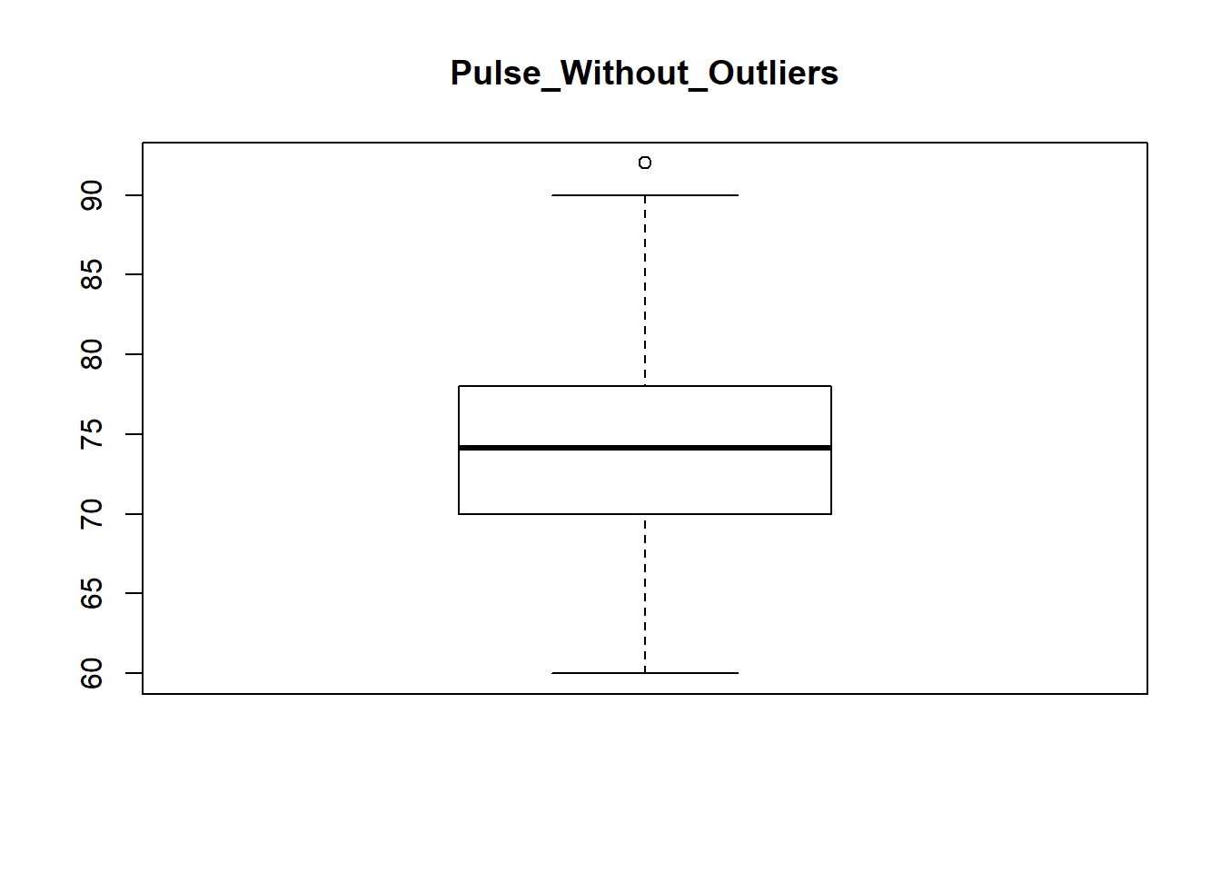
** So what happened here?? We are still able to see dots in boxplot!! Answer to this is though there are dots in boxplot, but we cann’t remove more data than that, because it will result in forging data, which will hamper the correct analysis of data. This happens a lot when you are working on large dataset, so keep in mind that not all the outliers can be removed
** Though if we don’t want them we can simply delete the data but it will result in data loss. So its not a good practice to delete them.
Now we will repeat same process for other three variables too.
- For variable Wr.Hnd
quantile(survey$Wr.Hnd, 0.05, na.rm=TRUE)## 5%
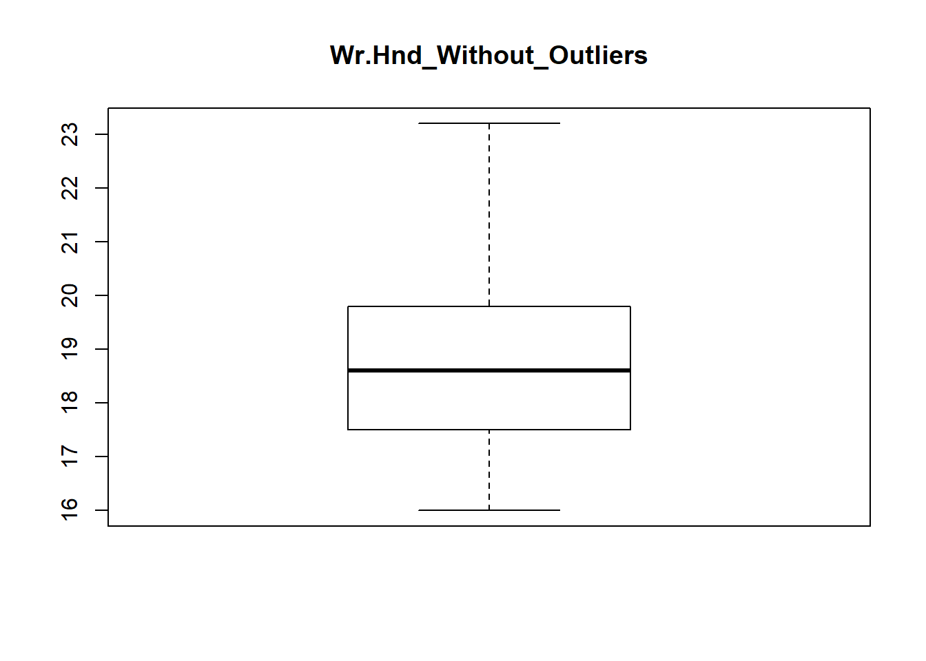
## 16survey$Wr.Hnd <- ifelse(survey$Wr.Hnd < 16, 18.84, survey$Wr.Hnd)
summary(survey$Wr.Hnd)## Min. 1st Qu. Median Mean 3rd Qu. Max.
## 16.00 17.50 18.60 18.84 19.80 23.20boxplot(survey$Wr.Hnd, main="Wr.Hnd_Without_Outliers")
- For variable NW.Hnd
quantile(survey$NW.Hnd, 0.05, na.rm=TRUE)## 5%
## 15.5quantile(survey$NW.Hnd, 0.95, na.rm=TRUE)## 95%
## 22.22survey$NW.Hnd <- ifelse(survey$NW.Hnd > 22.22, 18.53, survey$NW.Hnd)
survey$NW.Hnd <- ifelse(survey$NW.Hnd < 15.5, 18.53, survey$NW.Hnd)
summary(survey$NW.Hnd)## Min. 1st Qu. Median Mean 3rd Qu. Max.
## 15.50 17.50 18.50 18.52 19.50 22.20boxplot(survey$NW.Hnd, main="NW.Hnd_Without_Outliers")

- For variable Age
quantile(survey$Age, 0.95, na.rm=TRUE)## 95%
## 30.6836survey$Age <- ifelse(survey$Age > 30.6836, 19.22, survey$Age)
summary(survey$Age)## Min. 1st Qu. Median Mean 3rd Qu. Max.
## 16.75 17.67 18.58 19.17 19.83 30.67boxplot(survey$Age, main="Age_Without_Outliers")
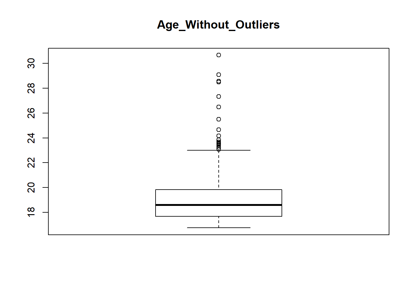
This is the same scenario that we faced while removing outliers from variable Pulse, but here the number of outliers is high. So in this scenario you can omit the data containing outliers for better results.
That’s all for this lecture, in next lecture we look into the things in a much deeper way.
Keep Learning!!!


Awesome post!
Thanks Judy!! We will keep posting such good posts so stay tuned and keep learning!!