Volatility Check in Returns charts
Hi All! In our previous tutorial, we had introduced stylized facts, what the five stylized facts are and had also covered stylized fact 1 – Distribution of returns – Is it non-Gaussian? In this tutorial, we will be covering stylized fact 2 – “Are Volatility clusters formed in returns chart?” and do Volatility Check in Returns charts using Python. New to this series? – Go to part 1 of Financial Analytics series to develop a good understanding on this.
Stylized Fact 2: Volatility Check in Returns charts
Let’s choose MSFT stock for our analysis. We’ll use yfinance to fetch stock data of MSFT.
# Importing the libraries
import pandas as pd
import yfinance as yf
import numpy as np
import matplotlib.pyplot as plt
# Downloading MSFT data from yfinance from 1st January 2010 to 31st March 2020
msftStockData = yf.download( 'MSFT',
                        start = '2010-01-01',
                        end = '2020-03-31',
                        progress = False)
# Checking what's in there the dataframe by loading first 5 rows
msftStockData.head()
# Checking what's in there the dataframe by loading last 5 rows
msftStockData.tail()
# Calculating log returns and obtaining column to contain it
msftStockData['Log Returns'] = np.log(msftStockData['Adj Close']/msftStockData['Adj Close'].shift(1))
# Checking what's in there the dataframe by loading first 5 rows
msftStockData.head()
# Using back fill method to replace NaN values
msftStockData['Log Returns'] = msftStockData['Log Returns'].fillna(method = 'bfill')
msftStockData.head()
# Line chart of log return series
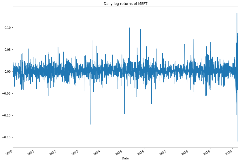
msftStockData['Log Returns'].plot(title = 'Daily log returns of MSFT', figsize = (14,10))
Thus, we can see that volatility clusters are formed in the line chart – there are some periods having higher returns and some periods have lower returns and they alternate forming a cycle of high-low-high. Thus, volatility doesn’t remain the same always.
So guys, we have just now explored Stylized fact 2 in this tutorial. In the next tutorial, we will explore stylized fact 3. Stay tuned! And don’t forget to subscribe to our YouTube channel.


One thought on “Volatility Check in Returns charts: FA9”