

Auto-correlation in Log Returns
Hi All! In our previous tutorial, we had covered Stylized fact 2: Are Volatility clusters formed in returns chart?. In this tutorial, we’ll continue exploring stylized fact and will go through Stylized fact 3: Is auto-correlation absent in returns? and will see if there is decreasing auto-correlation in log returns series using Python.
If you want to learn what are stylized facts, please go here. If you’re new to Financial Analytics, I suggest you start from here.
Stylized Fact 3: Auto-correlation in Log Returns
Before going ahead with this, let’s learn what is auto-correlation first.
What is auto-correlation?
If you go through a data series (column) and you seem to see a pattern in that series such that by looking at that pattern, you can predict the future values based on the past values, you infer that series is having auto-correlation in it. Auto-correlation is said to be present when values of a same variables of a data-set show some degree of similarity over consecutive time periods.
Types of auto-correlation
There are two types of auto-correlation:
- Positive auto-correlation
- Negative auto-correlation
Positive auto-correlation
In case of positive auto-correlation (first-order, auto-correlation can be nth order), first-order means that items are one value apart, we say that the correlation among successive observations is positive. In case of positive auto-correlation, if you plot time on x-axis and values of a variable on y-axis, you get an upward trend line, line moving upwards and having positive slope.
Negative auto-correlation
In case of negative auto-correlation (first-order, auto-correlation can be nth order), first-order means that items are one value apart, we say that the correlation among successive observations is negative. In case of negative auto-correlation, if you plot time on x-axis and values of a variable on y-axis, you get a downward trend line, line moving downwards and having negative slope.
Auto-correlation in Log Returns – The Code
We’ll learn this by means of example, but first let’s start importing MSFT stock data via Python.
# Importing libraries
import pandas as pd
import yfinance as yf
import numpy as np
import seaborn as sns
import matplotlib.pyplot as plt
import scipy.stats as scs
import statsmodels.api as sm
import statsmodels.tsa.api as smt
# Downloading MSFT data from yfinance from 1st January 2010 to 31st March 2020
msftStockData = yf.download( 'MSFT',
                        start = '2010-01-01',
                        end = '2020-03-31',
                        progress = False)
# Checking what's in there the dataframe by loading first 5 rows
msftStockData.head()
# Checking what's in there the dataframe by loading last 5 rows
msftStockData.tail()
# Calculating log returns and obtaining column to contain it
msftStockData['Log Returns'] = np.log(msftStockData['Adj Close']/msftStockData['Adj Close'].shift(1))
# Checking what's in there the dataframe by loading first 5 rows
msftStockData.head()
# Using back fill method to replace NaN values
msftStockData['Log Returns'] = msftStockData['Log Returns'].fillna(method = 'bfill')
msftStockData.head()
Correlogram or Auto-correlation or ACF plot
We can find which auto-correlation exists in a series by means of a correlogram or ACF plot.
- On x-axis, we have lag which starts from 0 and shows auto-correlation of each value with itself. It, then, goes increasing from zero to the lag value you define.
- On y-axis, we have value of auto-correlation for each lag. For lag 0, the auto-correlation value will be 1. For lag 1, the auto-correlation value is actually between successive values – one value apart. For lag 2, the gap between two successive values will be 2 and so on.
- To plot the ACF graph, we use smt.graphics.plot_acf function of statsmodels library.
We will obtain the ACF curve of log returns series of MSFT stock data and see if it satisfies Stylized fact 3.
# Setting lags to 25, significance level to 0.05, confidence level to 0.95
fig, ax = plt.subplots(figsize=(14, 10))
acf = smt.graphics.plot_acf(msftStockData['Log Returns'], lags=25, alpha=0.05, ax = ax)
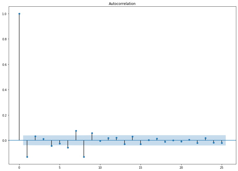
From the above graph, we can see that few auto-correlation values corresponding to lag values 1, 4, 6, 7, 8 and 9 are lying outside the confidence interval of 0.05 (region shaded in blue). After this, the auto-correlation values go on decreasing and become smaller and smaller.
From above, we can see that
- there is no auto-correlation in the log returns series.
- the auto-correlation values go on decreasing and become smaller and smaller.
So guys, with this I conclude this tutorial. In the next tutorial, we will cover Stylized Fact 4: Decreasing auto-correlation trend in squared/absolute returns. Also, subscribe to our YouTube channel where we explain all this in videos. Stay tuned!


One thought on “Auto-correlation in Log Returns: FA10”