

Decomposing Time-Series
Hi All,
In this tutorial, we will be discussing how to decompose stocks time-series into different components in order to have a good idea about the complexities of the time-series models and how to accurately capture them and account for them in our model.
Time-series components
Time-series components are of two types:
- Systematic components
- Non-systematic components
Systematic components
Systematic components can be modeled and described. They are always in tune.
Systematic components are broken down into 3 sub-components:
- Level: It is equal to the mean value of the series.
- Trend: It is defined as change in the successive values of the points of the time-series. This is generally characterized by a slope. If the change in the successive values is positive and the slope is positive, we get increasing trend, else we get decreasing trend.
- Seasonality: It is the deviation from the mean value that happen periodically in less than an year, quarter, month or week.
Non-systematic components
Non-systematic components cannot be modeled. They constitute of random values and hence, are consist of only noise.
Non-systematic components are broken down into one sub-component:
- Noise: It consist of random variation in data.
Models for Time-series decomposition
There are two types of models we employ to decompose time-series:
- Additive model
- Multiplicative model
Additive model
The additive model constitute of the following features:
- The additive model equation is y(t) = level + trend + seasonality + noise
- Linear model: Changes over time are consistent and grow or reduce linearly.
- Seasonality is linear and the frequency and amplitude of the series stay the same over time.
Multiplicative model
The multiplicative model constitute of the following features:
- The multiplicative model equation is y(t) = level trend seasonality * noise
- Non-linear model: Changes over time are non-consistent and grow or redice non-linearly.
- Seasonality is non-linear and the frequency and amplitude of the series keep on decreasing/increasing over time.
Decomposing time-series: Code
Let’s start by importing and loading the libraries. We will be importing 4 libraries:
- Pandas for data frame manipulation
- yfinance for downloading finance data
- statsmodels.tsa.seasonal for obtaining seasonal_decompose function for decomposing time-series and plotting the time-series decomposition charts. seasonal is the model under tsa (time-series analysis) module of statsmodels package.
import pandas as pd
import yfinance as yf
from statsmodels.tsa.seasonal import seasonal_decompose
import matplotlib.pyplot as plt
%matplotlib inline
The next step is to download the financial data-set from yahoo finance using download function of yfinance library.
- The date range we are selecting varies from 1st Jan 2020 till today.
- For that, let’s fetch today’s date using pandas first and store it in a variable.
- Then we will pass this to the end parameter of download function.
today = pd.Timestamp('today')
today
StockData = yf.download( 'MSFT',
                        start = '2020-01-01',
                        end = today,
                        progress = False)
Let’s now see what’s there in the data-set using head function.
StockData.head()
Let’s now check the variable statistics using the describe function.
StockData.describe()
Let’s also see if the data contains any missing values (which is not there, but still checking!).
StockData.isnull().any()
No missing values (as expected)! Let’s now start plotting the time-series decomposition chart. We are only interested in Adj Close, so we will obtain a time-series for the same. We will set freq parameter to b or to business days as trading happens on business days only. We will then use the forward fill method to fill N/As.
data = StockData['Adj Close']
data = data.asfreq('b')
data = data.fillna(method='ffill')
data.head()
Let’s now use data to plot time-series decomposition chart. We will use multiplicative model as in stock trading, nothing is linear, everything is non-linear.
res = seasonal_decompose(data, model='multiplicative')
fig, ax = plt.subplots(4, 1, figsize=(15,8), sharex=True)
res.observed.plot(ax = ax[0])
ax[0].set(title='MSFT Adj Close Observed', ylabel='Observed')

res.trend.plot(ax = ax[1])
ax[1].set(title='MSFT Adj Close Trend', ylabel='Trend')

res.seasonal.plot(ax = ax[2])
ax[2].set(title='MSFT Adj Close Seasonality', ylabel='Seasonality')

res.resid.plot(ax = ax[3])
ax[3].set(title='MSFT Adj Close Residuals', ylabel='Residuals')
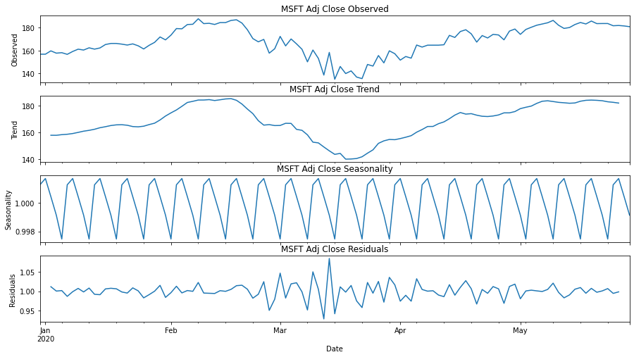
From above plot, we can see all the four components – Observed (Level), trend, seasonality and residuals (noise) for the Adj Close price.
- We can notice the trend to first increase, reach the top-most point then decrease, reach at the lowest level and then it started increasing again.
- We can also see that the seasonality pattern gets repeated after every week.
- There was very high level of noise in March (second week majorly).
- The noise component was stable during the starting of month of January and end of month of May.
So guys, with this I conclude this tutorial. In the next tutorial, we will be diving deeper into time-series analytics and will apply it on stock data and understand its application in the field of financial analytics. Please don’t forget to subscribe to our channel, ML For Analytics, where we are teaching all this in our videos. Stay tuned!


How can we identify that , the
Seasonality is getting repeated weekly ?